Will state national guard deployment reduce crime in D.C.?

Just over two weeks ago, the Trump Administration declared a “crime emergency” in Washington, D.C. in response to a former DOGE staffer getting injured in an attempted carjacking. As rationale for the emergency, the Trump Administration has described crime in D.C. as “out of control” and has named the District itself as, “by some measures, among the top 20 percent most dangerous cities in the world.” In January of this year, the Metropolitan Police Department announced that crime in D.C. reached the lowest it had been in 30 years. 

The Trump Administration has since taken control of the Metropolitan Police Department and deployed the District of Columbia’s National Guard in an effort to reduce crime in the city. Earlier this week, President Trump signed an additional executive order with guidance to staff the National Park Service with more police officers, hire additional attorneys to prosecute violent crime, and increase law enforcement training and resources, all to help crack down on crime in the District of Columbia.

The 1973 Home Rule Act gives the president the ability to invoke this kind of power by granting presidential control over the national guard in the District of Columbia and allowing presidential use of the local police during emergencies. These emergencies are permitted to last for up to 30 days without legislative authorization. 

The Home Rule Act has been invoked by presidents in the past, but never for reasons as broad and sweeping as crime. Prior to the current deployment in the District of Columbia, the most recent instance a president bypassed a governor to deploy state troops was to protect civil rights advocates in the 1960s. The use of the Home Rule Act and the deployment of the National Guard to fight everyday is unprecedented and is sure to face legal challenges and political pressure. 

Research from Brown University finds that in the past, military policing has done very little to actually reduce crime. The study focuses on Bogotá, Colombia, one of the cities President Trump has compared crime rates in the District of Columbia to. The study finds that military forces seldom decrease crime more than traditional police forces, and in many cases, crime rates end up higher than before once military forces leave. 

This data corroborates the concerns lawmakers in the District of Columbia have voiced. The National Guard does not receive the same type of training that local police officers receive on when and when not to use lethal force. Typically, the National Guard is used for more specific use cases, such as engaging in crowd control for protests, helping in the aftermath of a natural disaster, or controlling civil unrest. And, when it comes to handling crime, the National Guard acts more in-line with the military strategy of neutralizing dangerous threats than the police strategy of solving crime. In conjunction with recent reports of the National Guard carrying firearms, safety concerns in the District of Columbia are not without reason.

This poses the question: is deploying the National Guard an efficient use of resources to stop crime?

As of August 20th, six states have promised to send their National Guard troops to the District of Columbia: Louisiana, Mississippi, Ohio, South Carolina, Tennessee, and West Virginia. These troops will add more than 1,100 new soldiers to patrol the streets in the District of Columbia. 

Using FBI crime data, violent crime rates from these states compared to Washington, D.C. are shown in the chart below. 

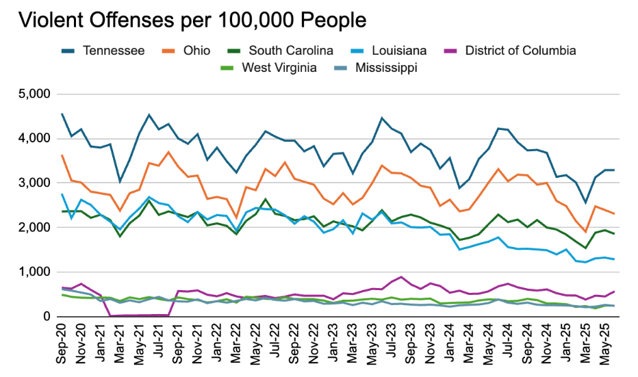
Out of the six states that have promised to deploy the National Guard to the District of Columbia, the rate of violent crime per capita in Washington, D.C. is only higher than two, West Virginia and Mississippi, both of which have fewer urban areas than the other states. Even if deploying the National Guard is an effective way to reduce crime, why aren’t states with crime rates higher than the District of Columbia deploying the National Guard in their own cities? In this case, it seems subnational policymakers have deferred local interests to federal interests.

Once troops are sent from the states, Washington, D.C. will have upwards of 2,100 troops deployed. More than half of these troops will be from states, and the total cost of these troops could exceed $1,000,000 per day, meaning that states could be collectively paying upwards of $500,000 per day to keep troops in the District of Columbia. At Scioto Analysis, we focus on state and local policymaking, and the question persists– is deploying troops to the District of Columbia a good use of state resources?

So far, the Trump administration has cited robberies down 46%, carjacking down 83%, and violent crime down 22% in the District of Columbia due to the executive orders. While the source of this data remains unknown, if these figures are accurate, it remains unclear if crime will continue to fall once the National Guard leaves, or if it will rise to levels at or higher than before the National Guard was involved, as historical precedence suggests it may.

Historically, effective strategies to reduce crime in the long-run focus on institutional change and local based efforts such as vocational training, extra police patrol, rehabilitation programs, incarceration for repeat offenders, and quality education for high-risk youth, while ineffective strategies include community mobilization against crime, high supervision based programs, and arrests for minor offenses. Policymakers may have more work to do if they wish to make further progress on crime in major U.S. cities.

Do markets stop at man?

Often when we talk about markets, we treat them like technology.

A history of the economy is often told like this: first, hunter-gatherers took food from nature and shared it among their tribes. Then, tribes began to trade with each other through barter systems. Agriculture brought stockpiling of resources and trade of those stocks. Then eventually cultures developed currencies, easing trade and creating markets like what we see today.

But what if there is something older than this? What if there are “deep markets” that go beyond not just history and prehistory, but beyond mankind? What if economics is not just a human phenomenon, but a biological phenomenon?

In this week’s Planet Money newsletter, economics journalist Alex Mayyasi covered research by Evolutionary Biologist Toby Kiers, who studies “markets” in sugar and nitrogen between soybeans and microbes.

Her theory: that the two were not leeching off each other, but rather were engaging in a free exchange. That meant they could withhold their side of the bargain if the other side was not held up.

So she put the theory to the test. She surrounded the microbes with air that did not include the nitrogen they provided to the soybeans. Kiers observed that when the soybeans were not provided the nitrogen, they did not provide sugars to the microbes. No payment, no product.

She found this played out in trades between plants and fungi, too. Plants in full sun were able to produce more sugars to trade than plants in full shade. The fungi gave more of their phosphorus and nitrogen to plants that provided them with more fats and sugars. The relationship was not parasitic–it was voluntary and reacted to shocks in supply.

With tools developed to track “nanoparticles,” Kiers teamed up with chemist Matthew Whiteside and biophysicist Tom Shimizu to follow these trading patterns. With these tools, they found that fungi save their phosphorus and nitrogen for times when sugars and fats from plants are more plentiful. This implies a “price” for trading that changes based on supply of resources.

According to Mayyasi, primatologist Ronald Noë has been documenting a phenomenon he calls “biological market theory,” that he first developed by observing monkeys trade food and grooming sessions like commodities. He notes changes in the “price” of mating as dictated by food offered during times with more or less balanced sex availability, cleaner fish who take advantage of larger fish when competition decreases, and comparative advantage developing between plant species in evolution as examples of markets developing in biological settings.

But how could this be? Don’t we know that human beings make decisions based on rational thought, weighing their strength of desire for a product against their personal resources?

Wait, do they do that?

Or do we make purchases on autopilot? Do we think through every single purchase we make or do we sometimes buy things bounded by general large bounds for reasonability. If I go to a food stand at a soccer game, I want to buy a hot dog. I will pretty much pay what they ask me for it unless it is extremely expensive. But really I’m just going to go up and give them my money and take what they give me. Their price is constrained not by my choice, but by the hundreds of people all making hunch decisions about what would be too much and walking away if it is too much to pay.

In Mayyasi’s words, “brains are overrated.” We’re not that far off from fungi: we want things and we have resources to trade for them. The mechanism by which fungi and plants make these decisions to trade is mysterious, but so is the neurological process that governs our economic decision making. From an objective, behavioralist standpoint, the two do not seem that different from one another.

This matters to me as a public policy analyst. When conducting cost-benefit analysis, our goal is to estimate how a public policy will change the economy, including how much resources will grow overall and how they will be distributed throughout the economy. When the welfare of non-human animals is raised, the first thought that comes to mind is this: non-human animals don’t take part in markets! How could you value the impacts of a public policy on their markets if they don’t exist?

But they do, and this market behavior stretches beyond non-human animals into plant and even fungal populations. We observe it happening, with populations exhibiting economic behavior that conforms to models eerily similar to that we see among human populations in markets much more familiar to us.

What does this mean for the public policy analyst?

First, it means that we are likely missing key stakeholders when we are conducting cost-benefit analyses. If changes to air quality can disrupt markets in trade between plants and fungi, what other changes to ecosystems come about from changes in public policy?

Second, this means analysts have a tall task ahead of them when it comes to monetizing these impacts. If fungi reproduce at lower rates when nitrogen content in the air reduces in quantity, what does this translate into in dollar terms? Our traditional approach to valuing an impact like this would be to find out how much this impacts human welfare, which is one way to value this. But is it worth valuing fungi in and of themselves? Surely the fungi are valuing their own reproduction since they are optimizing toward reproduction. How do we measure this against other goods in society like health and consumer goods that human beings establish a willingness to pay for through market activities?

I do not have all the answers to these questions. I do know, though, that there is work to be done. The more research uncovers truths about how life interacts with each other, the more certain I become that the line we draw between man and other life on earth is arbitrary and convenient more than scientific and indisputable. Science will keep pushing us to consider the larger impacts of our public policies. It is up to us to listen and to do the hard work of incorporating these broader impacts into our models.

Ohio economists believe BLS turmoil will hurt Ohio economy

In a survey released this morning by Scioto Analysis, 10 of 14 economists agreed that reduced trust in Bureau of Labor Statistics estimates will hurt economic development in Ohio. This comes after the firing of Commissioner Erika McEntarfer and subsequent appointment of E.J. Antoni from the Bureau of Labor Statistics has raised concern about the independence and reliability of Federal employment statistics.

As Curtis Reynolds from Kent State wrote “One of the hidden backbones of the US economy is the quality of economic data.  That provides investors - both in the US and from other countries - with reliable data for making decisions.  A belief that the quality of the data has decreased or is now being manipulated/manufactured for political gain will undermine confidence in the entire US economy.”

One economist who disagreed was David Brasington from the University of Cincinnati, citing challenges the Bureau of Labor Statistics has had recently in their survey response rates “I disagree with the premise.  If the new director makes the BLS use more updated models, trust in the numbers could increase.  Current BLS surveys have 45% completion rate compared to 95% in the past.”

Additionally, 10 of 14 economists agreed that reduced trust in Bureau of Labor Statistics estimates will increase the importance of state-level economic data. This does come with additional challenges of state’s having potentially differing methods, as Kathryn Wilson notes “Yes, but relying more on state-level data is a costly and an uneven substitute. If states vary in their ability or willingness to invest in high-quality data collection, the result will be inconsistent and less useful than national statistics. The costs of duplicating efforts at the state level would be significant, and there’s the added risk that state-level data could become further politicized along partisan lines.”

The Ohio Economic Experts Panel is a panel of over 30 Ohio Economists from over 30 Ohio higher educational institutions conducted by Scioto Analysis. The goal of the Ohio Economic Experts Panel is to promote better policy outcomes by providing policymakers, policy influencers, and the public with the informed opinions of Ohio’s leading economists. Individual responses to all surveys can be found here.

How does working from home impact the labor force?

Since the COVID-19 pandemic, significantly more people have been performing their jobs remotely instead of going into an office. Work-from-home policies have largely stuck around since the COVID-19 related restrictions have been lifted, changing the way people across the country work. 

Some of the effects of this are easy to see. Downtowns that used to be full of office workers are more sparse. Commuting patterns have changed However, we are only just beginning to understand what these policies have done to impact the labor market. 

A recent working paper from the National Bureau of Economic Research by Emma Harrington and Matthew Kahn looks at one outcome that comes from increased work from home opportunities: a reduction in the motherhood penalty, the career setbacks and earning disadvantages often experienced by women after having children. 

The motherhood penalty can result in a variety of negative outcomes for mothers in the labor force, including slower career progression, fewer opportunities for promotions, and lower overall earnings compared to their male counterparts and women without children.

One crucial aspect the researchers considered is who chooses to work from home when the option is available. It's not simply a matter of everyone transitioning to remote work equally. Factors such as the nature of the job, individual preferences, and household circumstances likely play significant roles in determining who takes advantage of location flexibility. Understanding these choices is essential for accurately assessing the broader impacts of work from home policies.

The authors’ analysis focused on technological advancements that made remote work feasible in various college degree fields even before the pandemic. By examining how the potential for working from home in different occupations influenced employment gaps for mothers, they uncovered compelling evidence of the impacts of work from home on the motherhood penalty. 

Their findings suggest that increased opportunities for remote work actually narrowed the employment gaps between mothers and others in the workforce. This effect was particularly pronounced in careers that have traditionally been considered less family-friendly such as finance and business. These are jobs that traditionally have longer and less flexible hours. 

An interesting finding from this paper is that mothers who work from home use their added work flexibility to take care of their children. For example, it’s easier to pick a kid up from school if you don’t have to leave and then return to the office. 

One question this raises for me is whether or not work-from-home policies might lead to fathers taking on a more even share of the child care responsibilities? Studies have found that women are more likely than men to be called by schools, which can lead to labor market challenges for women. If more men work from home, perhaps some of these external norms might begin to shift in such a way that helps further balance the duties of childcare.

While the long-term consequences of the widespread shift to working from home are still unfolding, research like this suggests some potentially positive outcomes. The increased feasibility and acceptance of remote work may offer a pathway to a more equitable labor market, where mothers are better able to maintain successful careers without facing the traditional penalties associated with balancing work and family life.

What would universal prekindergarten do for Ohio’s workforce?

What do Georgia, Oklahoma, Vermont, and West Virginia have in common? 

Despite the wide range of geography, politics, and demographics between these four states, they share a specific statewide policy in common: each has a universal prekindergarten system currently in place.

Over the past few decades, interest in prekindergarten enrollment among economists and education researchers has grown. Randomized controlled trials of high-quality prekindergarten programs conducted in the 1960s and 1970s have shown positive long-term outcomes for labor market earnings, health, and criminal justice involvement.

Researchers like Nobel Prize Winner James Heckman and Leading Economic Development Economist Timothy Bartik have used these findings to estimate the long-term economic benefits of investing in early childhood education, coming to the conclusion that early childhood is one of the best times to invest in education.

According to prekindergarten enrollment data compiled by U.S. News and World Report, Ohio is currently #37 in the country for prekindergarten enrollment, behind states like Alabama, Arkansas, Louisiana, Missouri, and New Mexico.

In April, my firm Scioto Analysis released a cost-benefit analysis we conducted on universal pre-kindergarten. In this analysis, we used results from a study conducted by the Washington State Institute for Public Policy to estimate what the benefits of a universal prekindergarten program would be for Ohio.

We estimated that increased lifetime earnings, reductions in criminal justice costs, and savings in special education would produce about $3.80 in benefits for every $1 of costs of the program.

Universal prekindergarten would not be a small investment for the state. According to 2023 American Community Survey data, Ohio has about 650,000 children under age 5. This means expanding prekindergarten to children age 4 would mean offering it to about 130,000 children and expanding it further would mean providing it to even more. Covering everyone would cost more than a billion dollars.

It is easy to get scared off by sticker shock by programs like this, but policymakers should take into account the impact this spending has on local economies. These funds will go toward paying prekindergarten teachers, who then have resources they can spend in the economy.

They also compare similarly to spending on vouchers for private schools, which often function as a windfall for parents already sending their children to private school rather than an incentive for children to enroll in high-quality programs.

Since the COVID-19 pandemic led to a nationwide reduction in workforce due to early retirements, layoffs, and untimely deaths, workforce has dominated so many of our state and local economic development conversations.

Investment in early childhood education is a strategy to build today’s education workforce and tomorrow’s broader workforce. As Timothy Bartik shares in his book “Investing in Kids,” high-quality universal early childhood education programs have returns to local wages that are on the scale of high-quality tax incentive programs for businesses.

A state that wants to build its long-term workforce needs to look to training people across all years of life. That means investment in postsecondary and technical education, K-12, but crucially early childhood.

Tomorrow’s workforce depends on decisions made, or not made, by policymakers today.

This commentary first appeared in the Ohio Capital Journal.

Why doesn’t the Official Poverty Measure adjust for geographic cost of living?

This week, the Ohio Association of Community Action Agencies released their 2025 State of Poverty Report, their annual report on poverty in the state of Ohio. One of the points that caught my attention in the report was Ohio’s listing as the 15th-highest poverty rate in the country with 13.2% of Ohio residents living under the federal poverty line.

These numbers come from the American Community Survey, which says that Ohio’s poverty rate was 13.3% in 2023 using 2023 survey data, so within the margin of error of what the Ohio Association of Community Action Agencies reports. It seems like their numbers are correct, but using the official poverty measure does mask some important distinctions between Ohio and other states that I would like to talk about.

Each year, when the United States Census Bureau releases their American Community Survey results, they also release a report called “Poverty in the United States” that details the poverty statistics of the previous year. One of the tables they release with the report is a table that shows state-by-state statistics for poverty based on two separate measures: the official poverty measure and the supplemental poverty measure.

We have written about different poverty measures plenty in the past but I will give you a rundown of the difference between these two measures. The Official Poverty Measure is based on Mollie Orshansky’s Great Society threshold of the cost of a thrifty food plan times three. In the 1960s, the average American household spent about a third of their income on food, so Orshansky reasoned that a good measure of “poverty” would be whether the household income does not exceed the resources to pay for three times a bare-bones food plan. The federal government agreed and that measure has stood, adjusted for inflation, for the past sixty years.

In the 1990s, however, a group of researchers were convened by the National Academies of Arts and Sciences to study and improve the federal poverty measure. In their report, this group of researchers addressed problems with the Official Poverty Measure.

The three main problems were as follows. First, the cost of food had plummeted in the United States over the past thirty years due to agricultural science advances. At the same time, health care and housing costs were on the rise. This challenged the idea of “the cost of a thrifty food plan times three” as a reasonable basis for setting a poverty threshold.

Second, the Official Poverty Measure only used pre-tax income to measure household resources. With the expansion of the social safety net and the role of taxes in household budgets, resources given and taken by the government have a substantial impact on poverty rates. The Official Poverty Measure ignores this.

Third, the Official Poverty Measure sets the same poverty threshold for every household in the United States, with the exception of separate thresholds for Alaska and Hawaii. This means someone living in San Francisco is expected to need the same amount of resources as someone living in rural Oklahoma.

The researchers proposed a new measure that ties thresholds to average consumer spending rates, factors in taxes, transfers, and living expenses, and adjusts for geography. The report then sat on a shelf until 2009, when New York City started calculating the New York Poverty Measure. The Census Bureau soon followed, developing the Supplemental Poverty Measure to estimate poverty nationwide. Scioto Analysis’s Ohio Poverty Measure is a version of this measure.

When you are seeing poverty rates cited, you are almost certainly seeing Official Poverty Measure rates. Even though these numbers are not as favored by poverty researchers as the Supplemental Poverty Measure numbers, they are still the numbers that are used for federal resource allocation, so they get top billing.

And so we see this in the Ohio Association of Community Action Agencies report. Ohio is good for 15th highest poverty rate in the country…under the Official Poverty Measure. This is one-year data from the American Community Survey, but it is a little more alarming than from three-year data reported by the United States Census Bureau in their “Poverty in the United States: 2023” report–in that report, Ohio was ranked 21st in the country for poverty.

Under the Supplemental Poverty Measure, though, the story is different. After adjusting for local cost of living, tying costs to average spending, and factoring in taxes and transfers, which the Supplemental Poverty Measure does, Ohio plummets from 21st in the country in poverty to 36th, dropping it from the middle of the pack for poverty to a state with below-average poverty rates. This 15-place drop is shared with Iowa (which drops from 33rd under the Official Poverty Measure to 48th under the Supplemental Poverty Measure) for the largest drop in ranking in the country when looking at the Supplemental Poverty Measure rather than the Official Poverty Measure.

When using this measure that adjusts for local conditions, states like Iowa, Ohio, New Mexico (2nd to 16th-highest poverty) and Maine (39th to 51st-highest poverty, ending up better than all states and D.C.) drop in the rankings due to lower costs of living. Meanwhile, high-costs states like New Jersey, Maryland, and Colorado, which are 44th, 41st, and 47th respectively under the Official Poverty Measure, catapult into the middle of the pack at 20th, 18th, and 26th under the Supplemental Poverty Measure. Large, relatively high-cost states of California, Florida, and New York increase from merely above-average rankings of 19th, 15th, and 17th highest poverty in the country under the Official Poverty Measure to 1st, 4th, and 6th respectively under the Supplemental Poverty Measure.

Cost of living matters. A dollar in Southeast Ohio is not the same as a dollar in the San Francisco Bay Area. If we look at a measure like the Supplemental Poverty Measure, we will get a lot closer to understanding what true relative differences in poverty are from state to state. And that matters. Designing antipoverty policy around good data is important because it will help us bring the end of poverty more quickly and with less pain. And isn’t that what antipoverty policy is for?

What is a market failure?

At Scioto Analysis, our core specialty is microeconomic analysis of public policies. We use this lens because microeconomics provides a framework for understanding how individuals, households, and firms make decisions in response to changing market conditions. 

One of the most important models we use is basic supply and demand. How people react to changes in market prices can tell us a lot about underlying economic conditions. Understanding these markets is essential.

In a competitive market, the price of a good will eventually reach an equilibrium such that supply equals demand. Given the assumptions of a competitive market, this has the fortunate side effect of maximizing total surplus in the market. In other words, an intervention in the market will result in less overall value existing in the economy. 

Unfortunately, perfectly competitive markets don’t really exist in the real world. Because of this, it’s worth understanding what the gaps are between real markets and ideal markets. If we understand why markets aren’t working at maximum efficiency, then we can consider ways to address those issues and create more value for society. 

One of the most common and important market failures is the existence of externalities. An externality is some effect that occurs when a good is consumed or produced that affects third parties to a market transaction. Classic examples are pollution from a factory or secondhand smoke from cigarettes. 

If an externality is the only market failure, then that market actually does operate completely efficiently for the buyers and sellers who participate. The issue is that because people outside the market are harmed (or helped in some cases) by that market activity, overall wellbeing might actually increase if less of that good was consumed. The private equilibrium does not align with the social equilibrium.

Another important market failure is information asymmetry. This occurs when one side of the market has some private information that allows them to take advantage of the other. A common example of this is a shady used car dealer who intentionally hides defects in order to sell poor cars at high prices. 

A less nefarious example of imperfect information is if a market participant is unaware of viable substitutes. A buyer might not know that other sellers of a good might offer better prices or quality, or a seller might not know their product could fetch a higher price if they sold to other clients. 

Another significant market failure arises from public goods, which are defined by two key characteristics: they are non-rivalrous and non-excludable. Non-rivalrous means that one person's consumption of the good doesn’t prevent another person from consuming it. Non-excludable means it is impossible or very costly to prevent someone from consuming the good once it has been produced, even if they haven't paid for it.

One example of a public good is a city park. One person walking their dog through the park doesn’t prevent someone else from having a picnic, and it isn’t possible to keep people who don’t help pay for the park’s maintenance from enjoying the greenspace.

Because of these characteristics, public goods are often underprovided by the private market. This is due to the "free-rider problem," where individuals can benefit from the good without paying for it. A private company would struggle to make a profit providing public parks because they can’t reasonably make people pay. As a result, the government typically steps in to provide public goods, funding them through taxes.

One final important market failure is the existence of monopolies. In economic theory, monopolistic firms have the ability to extract greater surplus for themselves at the expense of lower surplus for consumers plus an additional deadweight loss. In other words, they take an extra slice of the pie at the cost of throwing the rest in the garbage. 

Because of this, monopolies are generally illegal. However, there are cases where it actually makes sense to allow firms to have monopoly power. These are called natural monopolies, and they occur when the upfront costs of entering a market as a seller are extremely high or where there are significant economies of scale. 

The most common example is local utility providers. It would be extremely expensive for more than one company to build a major power plant and transmission infrastructure, so in many places single firms are allowed to manage all the utilities. Where I live in St. Paul, Minnesota, we have Xcel Energy. These firms need to be closely regulated since they don’t have natural competitors to encourage them to act in a socially optimal way.  

Market failure is a key consideration for policy analysts like us. They give us guidance for where government can improve markets through tools like taxes, subsidies, public goods provision, and regulation. This provides us with a roadmap for how government and markets can work together to improve social welfare as a whole.

What is Pigouvian Taxation?

This summer, my favorite podcast Planet Money is doing its most recent version of an “economics 101” series they have done the past couple of years called Planet Money Summer School.

First, if you don’t listen to Planet Money, start. It is the best public policy podcast out there, and it isn’t even a public policy podcast. The podcast started as a National Public Radio show in the wake of the Great Recession. The idea: talk about economics…in a way that isn’t completely boring. In this way, Planet Money is trying to do the same thing Scioto Analysis is–though they are admittedly a little better at it than we are.

Why I call Planet Money the best public policy podcast out there is that they are constantly talking about the public policy implications of topics they cover. I don’t think this is necessarily something the reporters on the show set out to do initially, but I think it’s a natural outgrowth of reporting on the economy. It is impossible to cover the economy without covering how the public sector interacts with it. As much as people want to paint the U.S. economy as a privatized economy, the economy is decidedly mixed, with the public sector intervening in private markets through regulations, subsidies, taxes, enforcing property rights, certification, and a number of other avenues.

This summer’s Planet Money Summer School is focused specifically on this topic: how government interacts with the economy. This has made it a bit of a crash course in public policy analysis, especially given that economics is our main framework for conducting public policy analysis.

I was surprised about this when I first enrolled in graduate school. I do not know exactly what I was expecting when I first enrolled in the University of California, Berkeley’s Graduate School of Public Policy, but two courses of microeconomics was not exactly what I thought I would encounter. I found myself confused by why we spent so much time on economics and not much time on philosophy and political economy.

Ultimately, I came around to it. Aaron Wildavsky, the original founder of Berkeley’s public policy school, settled on a curriculum of microeconomics and statistics when starting the school, figuring an education in accounting and management would be too redundant with education students would learn on the job and that an education in political economy and philosophy would be too abstract to be useful to aspiring analysts. Microeconomics and statistics allowed analysts to construct models that could be used to understand how public policies work and what they do to the economy and, by proxy, people’s lives.

This Planet Money Summer School has been a great reminder of this to me. The episode I listened to the other day was on taxes. The episode was over 37 minutes long–quite long for a Planet Money episode. But this topic is so important. In the United States, one in every four dollars in the economy is collected in taxes, filtering through the public sector. The way these taxes are designed has a significant impact on the economy as a whole.

One segment of the story made my ears perk in particular: the segment covering Pigouvian taxes. Pigouvian taxes are taxes named after Early 20th-Century Economist Arthur Pigou, a father of welfare economics. He developed a theory of market failure that undergirds many public policy and public sector economics, the theory of externalities.

The main thrust of the theory of externalities is that there are certain economic transactions that happen where the consumer and the producer are not the only parties affected by the transaction. If someone purchases electricity from a coal-fired power plant, the consumer pays the producer for energy. This means the consumer gets energy and the producer gets money. Children who play in the park downwind from the power plant get the nitrous oxide and particulate matter emissions from the plant in their lungs.

From an economic standpoint, this means that the social costs of the transaction exceed the private costs. So while markets are efficient systems for allocating resources when goods are purely private, when trade in goods generate these external costs (“externalities”), social costs exceed private costs, incentivizing producers to overproduce and consumers to overconsume the good due to costs being unloaded on third parties.

Pigou had a theory for how to fix this problem: tax goods that have negative externalities. This tax then brings the private cost in line with the public cost, making the market efficient, and generating revenue for the public sector as a bonus.

This theory has gone on to be incredibly influential in public policy over the past century, being the major theory undergirding carbon taxes, providing a framework for taxing secondhand smoke and the external costs of alcohol, and inspiring contemporary policies like Manhattan’s new congestion fee. These are all forms of Pigouvian taxation.

What I found most compelling about this Planet Money episode, though, was the suggestion for a Pigouvian tax put forth by guest Derrick Hamilton.

I first came across Derrick Hamilton when he came to my home of Columbus, Ohio to serve as the director of the Kirwan Institute, a data and racial equity institute at Ohio State University. At the time, he was talking about baby bonds, the idea that the public sector should put a certain number of dollars toward every new child that then grows in value until they are awarded it at age 18.

During the Planet Money episode, he was asked what Pigouvian tax he would want to put in place. His answer? Junk mail. You get mail sent straight to your home that (1) is not good for the environment, and (2) requires you to go through the work of sorting and throwing away. Both of these are external costs incurred by society not currently captured by junk mail.

I hate junk mail. I hate that we have advanced to the point where we can do most of our mail communication electronically and yet I still have a chore I have to do daily of throwing away unwanted solicitations in my mail. This seems like a fair use of our tax system, and a smart one, too. Why not give us our time back, save the environment, and raise more public funds to boot?

Pigouvian taxation is an incredible tool. I would love to see it unleashed on one of my worst enemies: unwanted paper in my mailbox. Can you think of a new Pigouvian tax we could put in place?

New California Poverty Measure statistics show what poverty is like in the Golden State

Last week, my colleague Rob Moore wrote about relative poverty measures and how we might benefit from changing the way we calculate poverty. At Scioto Analysis, we calculate our Ohio Poverty Measure, a version of a relative poverty measure focused on the state of Ohio. We conduct this as a part of our social bottom line work, updating it when we can find time between client projects.

Our project was based on work done in other places such as Wisconsin, New York City, and California. The main difference between these reports and the Supplemental Poverty Measure is that these measures use American Community Survey data rather than Current Population Survey data. 

The American Community Survey is much larger than the Current Population Survey, but it doesn’t have as much detail. This means that researchers get the additional geographic resolution needed in order to construct these more local poverty measures, but they need to create models to estimate some of the information that is not included in the American Community Survey. 

Recently, the updated data for the California Poverty Measure was released. I wanted to highlight some of the takeaways from this report to help demonstrate why it’s important to have such local poverty data.

In 2023, 9.8% of working Californians between ages 25 and 64 (about 1.5 million people) were living in poverty. The California Poverty Measure poverty threshold for that year averaged $43,990 for a family of four, but varied widely depending on location.

About half of all working adults in poverty were employed full-time for the whole year, and their poverty rate was 6.7%. For those working part-time all year, the rate shot up to 23.6%, and for those working only part of the year, 18.4%. The expiration of pandemic-era supports contributed to a 1.1 percentage point increase in the worker poverty rate from 2022.

An additional 2.3 million people were near poverty, with incomes between 100% and 150% of the poverty line. Certain industries and occupations had especially high poverty rates. Agriculture and service sectors like administrative services, leisure and hospitality, and other services all saw rates above 18%. Among occupations, fishing, farming, forestry, and building maintenance topped the list, with one in four workers in poverty.

Geography matters, too. Southern coastal California had some of the highest poverty rates for working adults, with Los Angeles County at 12% and Orange County at 11.3%. Regions like the Sacramento area and Northern California had much lower rates, around 6.6%. In high-cost regions, even full-time employment was not always enough to escape poverty, pointing to the interplay of wages, expenses, and safety net accessibility. These geographic insights are unique among these types of poverty measures.

Family structure also shapes poverty risks. Most poor working adults live with other adults, often with children. Poverty is particularly acute for single parents without other adults in the household, nearly one in four are in poverty. For single adults without children, the rate is lower but still significant.

The California Poverty Measure shows that earnings account for about 80% of poor workers’ resources. These are supplemented by programs like the Earned Income Tax Credit and CalFresh. Without these supports, another 4% of workers would fall into poverty.

For policymakers, these findings demonstrate that higher wages, more hours, and career advancement are important but not sufficient on their own. Access to child and elder care, healthcare, and education and training all play a role in whether work leads to economic security.

We plan on updating our own Ohio Poverty Measure sometime in the near future. Hopefully we will one day have the capacity to make regular updates so we can get these types of insights in real time for Ohio. 

Ohio lawmakers could focus on increasing incomes instead of minor, ineffective property tax changes

On July, Republican lawmakers in the Ohio House of Representatives voted to overturn Republican Gov. Mike DeWine’s veto of a line in the state budget that would ban certain types of levies from being put on the ballot by local governments or school districts.

The reason House members thought this was so important that they needed to get together and have this vote even when their chamber was closed for renovation was because they saw this as a way to reduce the burden of property taxes.

In the wake of COVID-19, global supply chain disruption, a contraction of building materials, and changes in demographics caused substantial shifts in housing supply.

Many in Ohio have seen the value of their home increase precipitously in the years since 2020, especially in 2022-2024.

With three-year valuations coming in, many were hit with sticker shock of their new property taxes, and state lawmakers leapt into their fighting stances, ready to find a way to reduce the impact of property taxes on households.

The Ohio General Assembly commissioned a committee to study ways to reduce the burden of property taxes. This led to a series of provisions in the new state budget trying to reduce the burden of property taxes in the state.

The provision that was vetoed and the focus of the Ohio House override is focused on a specific type of levy: an emergency or replacement levy.

This is still a levy that has to go before voters, the same way any other property tax levy does.

The argument made by House members on the floor was that by banning the use of the phrase “emergency” or “replacement,” voters would not be “tricked” into voting for property taxes they didn’t believe in.

So basically, the diagnosis here is that property taxes are so burdensome, at least partially, because people mistakenly vote for them.

Ultimately, these sorts of policy changes to the property tax system will do little to reduce the burden of property taxes.

Yes, legislators can now go to their constituents and say “Hey, I went out there and voted even as the House chamber was under renovation to deliver property tax relief to you.”

But these are small administrative changes to the types of property taxes that are being put before voters. They will do little to reduce the burden of property taxes.

It is worth asking the bigger question: are property taxes really the problem residents of Ohio are struggling with?

Or is the real problem that property taxes grew in a short period of time relative to incomes?

Because that is unlikely to happen again soon with interest rates high and the global supply chain for building materials at a new equilibrium.

There is good reason to believe that legislators are stuck fighting the last war around property taxes.

So what can policymakers do?

They can improve upon the system by moving from a property tax to a land value tax, which falls less heavily on low-income renters and does not penalize people for developing their land.

They can invest in programs like early childhood and K-12 education which improve incomes in the long-run or the earned income tax credit and child tax credit which would improve incomes in the short-run.

Or they can keep beating around the bush, making small changes to the property tax system that do little more than to complicate an already-complicated system.