Is it time to embrace relative poverty measures?

In 2019, Ajit Banerjee and Annie Duflo won the Nobel Prize in Economics. They won the prize for their work on poverty across the world, using rigorous experimental methods to understand the nature of poverty in some of the world’s poorest regions. 

In their 2011 book Poor Economics, Banerjee and Duflo share the results of an experiment to learn about the relationship between poverty and hunger. In this study, they went to people with the lowest of low incomes and asked them about calorie intake. They tracked what people were eating and how many calories they were consuming in their state of extreme poverty.

Their theory was this: if people with few resources have low caloric intake, they will increase their caloric intake as they receive money. So they tested it, giving people money and seeing how their caloric intake changed as they received this money.

A strange thing happened. Among people who received money, their caloric intake decreased when they received it. So people who had the least money in the world, given the chance to increase their caloric intake, actually decreased their intake of calories.

Well why was this? It turned out that people who were living with the lowest amount of resources in the world decided to change their diets when they received cash payments. Instead of just eating rice and lentils, they started to eat a meal or two a week of meat or fish. These meals have much lower calories per dollar than meals of just rice and lentils, but these low-income people preferred to have a little variety in their meals, even if it meant sacrificing calories.

This is one reason, among many, that the current Official Poverty Measure seems to be out of whack with our conceptualization of poverty in America. The Official Poverty Measure was developed by Mollie Orshansky, an economist working in the Social Security Administration during the Johnson Administration. At the time, the average American family spent about one-third of their income on food. For this reason, Orshansky believed an adequate income would be the cost of a thrifty food plan times three. The federal government agreed with her and it was adopted as the poverty threshold.

We still use this threshold as our measure for poverty today, adjusted for changes in cost of living each year by the Department of Health and Human Services. There are some problems with this measure, though. First, families spend much less on food today than they did sixty years ago because food costs much less. On the other side, families spend much more on health care and housing, which relatively cost more than they did sixty years ago. The official poverty measure also does not have adjustments for cost of living, so a household of four in rural Oklahoma has the same federal poverty measure threshold for poverty of about $32,000 as a family of four living in a flat in San Francisco.

More fundamental than these problems of changes over time, though, is this assumption that people below the federal poverty line will starve. Yes, food insecurity exists in the United States, but starvation is nearly nonexistent in the country. The reality of the poverty line is that we are not trying to define how much is needed to literally survive. There are plenty of people who live for years under the federal poverty line. What we are trying to define is how much is needed to live a dignified life.

The allure of a measure based on food intake is that it gives us a veneer of scientific reasoning. We look at Maslow’s hierarchy of needs (which I could write a whole other blog post on) and our eyes go straight to the foundation: we need food to survive. So let us calculate the cost of food and use that as a basis for this idea of what income people need to not die.

What Banerjee and Duflo show us is how much of a sham this approach is. We’re not getting any closer to a “survival” estimate by saying how much it costs to buy a thrifty meal plan. Even during Orshansky’s time, the federal poverty measure did not capture what we meant by “poverty.”

An alternate poverty measure that gets closer to the concept we really have when we talk about poverty is the Supplemental Poverty Measure. The Supplemental Poverty Measure is an improvement on the Official Poverty Measure that makes adjustments for geography and estimates the impact of public benefits and taxes on poverty rates. Most importantly, it pegs the threshold to average spending levels, implying that poverty is defined by the inability to spend within a range of average spending in the country.

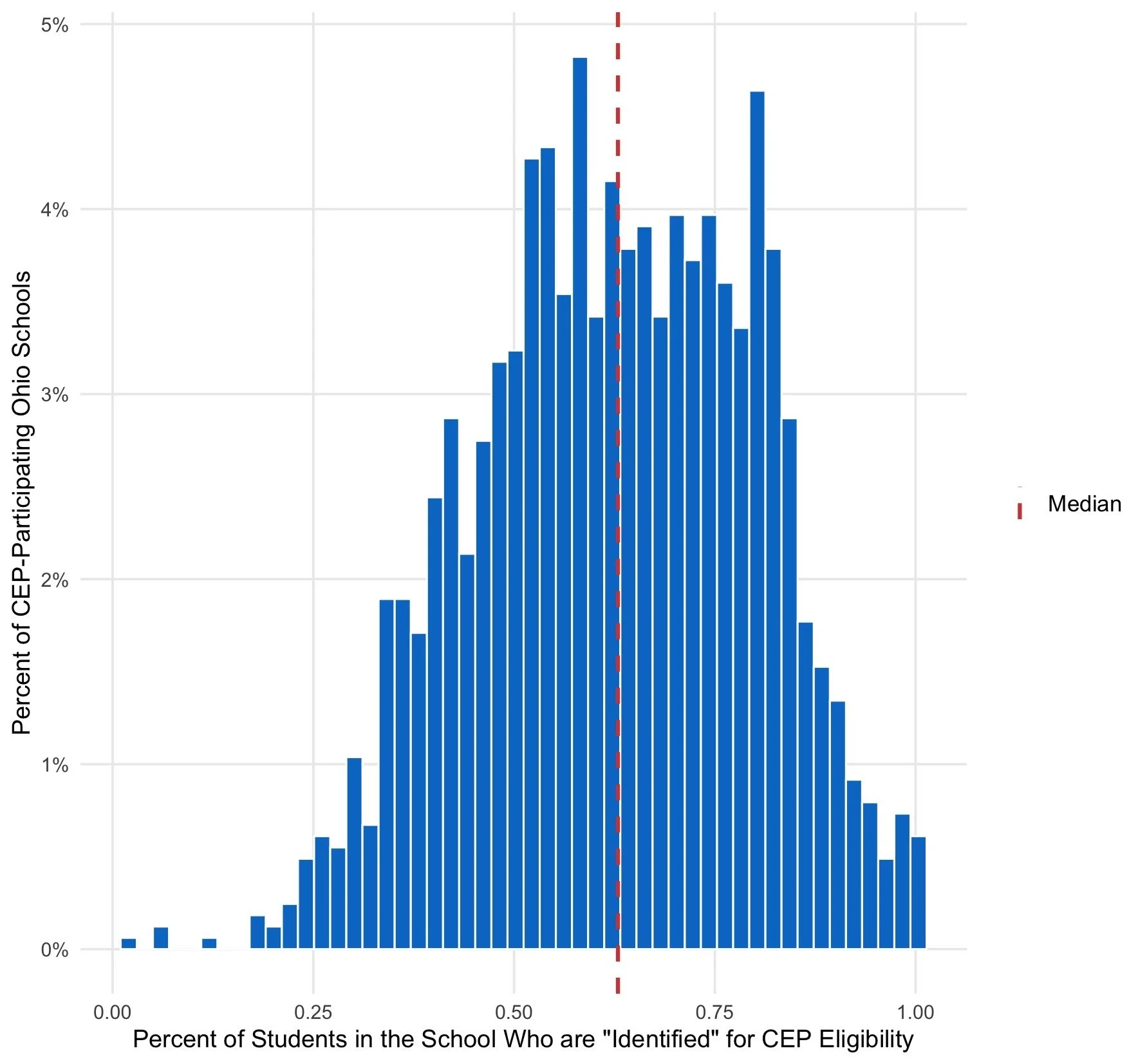
This is what we mean when we’re talking about poverty: does your ability to provide goods for yourself and your family fall far outside of the norms for your community? In our Ohio Poverty Measure, we make a similar estimate based on American Community Survey data, getting geographic precision that becomes even smaller than counties in populated parts of the state.

This line of reasoning, though, makes me even more interested in purely relative measures of poverty. A common measure of poverty, and the measure that is used by the Organization for Economic Co-operation and Development (OECD), is 50% of the median income. One thing I find attractive about the measure of 50% of the median income as the poverty measure is that it is incredibly easy to estimate anywhere. If you know what the median household income is for an area, all you need to do is divide it by two, then compare someone’s income to that. Then you know if they are in poverty or not.

Poverty will always be a contested concept. There are certain researchers at think tanks like the American Enterprise Institute who argue that poverty has almost completely disappeared in the United States, arguing that people consume so much more than they did during the Johnson era and that should be our measure for poverty. There are others who add up a list of items they believe make up household essentials and say if you can’t pay for these at market rates, then you are in poverty. These measures put the poverty rate at as high as half the U.S. population. 

Both of these definitions strain the definition of “poverty,” giving us answers to the question of who is in poverty that do not fit with our intuitions about what defines poverty. Ultimately, poverty is a socially-defined term. Having it connected to society through a relative measure is the most rigorous way to define poverty in line with the reality of how people see it in their communities.

What is the Community Eligibility Provision for school meals?

In the past decade, a new federal program has reshaped how over 27 million children across the country receive school meals. The Community Eligibility Provision allows schools with a large number of low-income students to serve free meals to all students, as an alternative to the traditional free and reduced-price meal system in the National School Lunch Program and School Breakfast Program. The federal government established the Community Eligibility Provision as part of the Healthy, Hunger-Free Kids Act of 2010, and the program became available nationwide beginning in the 2014-2015 school year. 

The Community Eligibility Provision has been a topic of hot debate. Advocates argue that the Community Eligibility Provision makes school meals more accessible and less stigmatizing for students in need, reduces schools’ administrative costs compared to the traditional school meals system, and improves students’ academic and health outcomes. These claims are generally supported by research, although the body of evidence is still relatively small since the Community Eligibility Provision is so new.

Critics, however, contend that the Community Eligibility Provision is an inefficient use of tax dollars, noting that some students in schools that participate in the Community Eligibility Provision come from higher-income families and do not need free meals. The Heritage Foundation’s Project 2025 agenda suggested that Congress should eliminate the Community Eligibility Provision and “restore [the National School Lunch Program] and [School Breakfast Program] to their original goal of providing food to K–12 students who otherwise would not have food to eat while at school.” Earlier this year, federal lawmakers considered reducing eligibility for the Community Eligibility Provision, but as of July 2025, that change has not been implemented.

The number of Ohio students whose schools participate in the Community Eligibility Provision has increased substantially since the program began. In 2015, 19% of Ohio students were in schools that participated in the Community Eligibility Provision. By October 2024, the number had risen to 40%, or 684,000 students across the state. The rise in participation is likely due to a combination of expanded eligibility, new methods for certification, and increased interest in providing free school meals to all students after the USDA temporarily provided universal free school meals nationwide during the Covid-19 pandemic.

Schools can apply for the Community Eligibility Provision individually or as part of a group through a Local Education Agency, such as a school district or charter school organization. For simplicity, I will refer to Local Education Agencies as “districts.” To be eligible to participate in the Community Eligibility Provision, at least 25% of the enrolled students must be “identified” with certain criteria. An “identified student” is any student who is automatically certified to receive free school meals due to household participation in other social safety net programs, such as the Supplemental Nutrition Assistance Program (“food stamps”) or Temporary Assistance for Needy Families. The number of “identified” students may be lower than the total number of students eligible for free meals, since not all eligible families participate in the safety net programs that are used for automatic certification.

Enrolling in the Community Eligibility Provision does not guarantee that a school or district will receive enough federal funding to provide free meals to all students. The federal government reimburses schools for enough meals to serve 1.6 times the “identified student percentage,” meaning the percent of students who meet the automated eligibility criteria described above. Thus, in order to receive federal reimbursement that covers free meals for all students, a school or district’s identified student percentage must be at least 62.5% (since 62.5% x 1.6 = 100%). Multiplying the identified student percentage by 1.6 helps provide coverage for low-income students who are not automatically identified through other safety net programs. 

If a school or district’s identified student percentage is less than 62.5%, they may need to supplement with local or state funding to provide free meals to all students. 51% of Ohio schools that participate in the Community Eligibility Provision have an identified student percentage greater than or equal to this threshold, although this statistic does not necessarily indicate whether the schools receive enough federal reimbursement to cover all students, since eligibility and reimbursement rates are often determined at the district level.

The plot below displays the distribution of identified student percentages across Ohio schools that participate in the Community Eligibility Provision. The median identified student percentage across schools is 62.9%. Some schools have identified student percentages lower than the 25% eligibility threshold, because they are enrolled in the Community Eligibility Provision at the district level and have a lower poverty rate than the other schools in their district. For example, the Columbus Gifted Academy has an identified student percentage of only 1.6%, but is enrolled in the Community Eligibility Provision because it is part of the high-poverty Columbus City Schools district. As noted above, the total number of low-income students is typically higher than the number of “identified” students.

Distribution of “Identified Student Percentages” Across Ohio Schools Participating in the Community Eligibility Provision

Plot generated with data from the Ohio Department of Education and Workforce; code available here.  

Beyond the Community Eligibility Provision, the State of Ohio has also expanded access to free school meals using state funding. Since 2023, Ohio reimburses schools to provide free meals to students who are federally eligible for reduced-price meals. In the 2025 legislative session, the Ohio Senate considered a bill to expand access to free school meals to all Ohio students, but the bill did not pass. Universal free school meals remain a topic of national conversation, so we may see other changes proposed in the near future.

For more on school meals, see our work on the history of school meals, school meals and student achievement, and universalfree school meals.

Ohio economists agree Medicaid cuts will have impacts beyond healthcare loss

In a survey released this morning by Scioto Analysis, 19 of 20 economists agreed that reducing Medicaid spending in Ohio by $37 billion over the next ten years will have significant economic ramifications in the state beyond loss of health insurance for current Medicaid recipients. This comes after the passage of HR1, the “Big Beautiful Bill Act.” KFF estimates that this bill will result in about $37 billion less being spent on Medicaid in Ohio.

Many respondents specifically identified the potential labor market impacts that cutting Medicaid spending could have. “Denying health care may reduce the supply of labor.  If people are unhealthy, they will not be able to work,” wrote Charles Kroncke of Mount Saint Joseph university. Bob Gitter of Ohio Wesleyan similarly noted “More sick time, potential job losses due to missed time at work, and potential closing of rural hospitals.”

Despite this, the 12 of 20 economists did not believe that these cuts would cause a severe recession in Ohio. “$37 billion over 10 years or $3.7 per year is about a third of a percent of Ohio's annual GDP, unlikely to create a recession, especially a big one. However, it could contribute to a recession caused by something more major,” wrote Christian Imboden of Bowling Green University. 

One economist who believed this would lead to a recession was Iryna Topolyn from the University of Cincinnati, writing “I am not certain about the severity of recession, but I am fairly confident that this cut will spur recession. The direct effect of reduced spending on medical services, amplified by the multiplier effect, will be observed in the short-run. Moreover, there will be economic loss due to sick days as a result of poorer health. Additionally, in the long-run there will be a negative effect of deteriorating human capital due to worse health outcomes.”

The Ohio Economic Experts Panel is a panel of over 30 Ohio Economists from over 30 Ohio higher educational institutions conducted by Scioto Analysis. The goal of the Ohio Economic Experts Panel is to promote better policy outcomes by providing policymakers, policy influencers, and the public with the informed opinions of Ohio’s leading economists. Individual responses to all surveys can be found here.

What is a land value tax?

A big policy discussion recently in Ohio has been about property taxes. They have become such a contentious project that one advocacy group has been pushing to abolish them in Ohio.

A few months ago, my colleague Rob Moore wrote an commentary exploring some of the alternatives to property taxes that could be used to replace the missing revenue should property taxes be abolished. Today, I’d like to talk more in-depth about one of those alternatives: a land value tax.

As the name suggests, a land value tax differs from a property tax by raising revenue from the assessed value of the undeveloped land on each parcel as opposed to the total value of the development of that parcel. This means that two neighbors that have to pay different property taxes because of the differences between their houses would have to pay the same land value tax since their undeveloped plots are essentially identical.

Economists are generally enthusiastic about this idea because it solves a major problem that property taxes have: they disincentivize people from making improvements to their property. 

This is not such an issue in properties where the residents own the property since they can internalize all this information and make an optimal decision. However, this creates problems in rental properties where the owners have less of an incentive to improve the living conditions. 

Those of you who are familiar with property tax research are probably aware that renters actually bear a large portion of the burden of property taxes, but they don’t bear 100%. This means that if property taxes go up as a result of some improvement, then a landlord would not get the full marginal benefit of the increased rents they would receive. If instead there was a land value tax in place, then making those improvements would not change their tax bill at all, and the landlord would have an increased incentive to make those improvements. 

It is interesting to consider what would actually happen in practice if property taxes were replaced with land value taxes. Lets assume that we want to have a revenue neutral land value tax, that is we raise the same total revenue with both. 

Property values are almost always higher than land values, so the land value rate would need to be higher in order to make up the difference. The city of Altoona, PA implemented a land value tax in 2002, and they found that the total assessed value of their land was one-seventh the assessed value of all the property, so their land value tax rate was seven times higher than the property tax rate.

If the land value tax rate is seven times higher than the property tax rate, then in order to figure out what this would look like for individuals we just need to determine what the difference is between the assessed value of their land vs. their property.

If the property is exactly seven times as valuable as the land, then they would pay the same amount of taxes under each scenario. If someone’s property is highly developed and is worth more than seven times the amount of the undeveloped land, then that person would end up paying less in their final tax bill. Finally, if the property is undeveloped or underdeveloped, then it would incur a higher tax bill under a land value tax. 

This is particularly important when thinking about completely undeveloped land. Speculative real estate investors can purchase undeveloped land and wait until real estate prices go up before selling it at a higher price to someone who is actually interested in developing it. If they had to pay land value taxes instead, they would be faced with much higher taxes in the interim, which could lead to those properties only being purchased by people with plans to develop them in the first place. In an urban setting where there isn’t enough land to go around, a land value tax changes the incentive structure and makes it more worthwhile to improve the quality of developed structures. 

Housing is becoming an increasingly important problem for local governments across the country. Land value taxes won’t solve every single problem, but they could be a better alternative to property taxes in some areas.

What is Moving to Opportunity?

The neighborhood a person is born in has a significant impact on their life trajectory. According to Census Reporter and the Centers for Disease Control and Prevention, children born in the communities of Avondale and Belvidere outside of Canton, Ohio can expect to grow up to have a median income of $92,000 and an average lifespan of 82 years. By contrast, the neighborhoods five streets over, Meyers Lake and Lakeview Terrace, face much bleaker prospects: their kids can expect to make about 40% less and live seven fewer years than their neighbors just a 10 minute drive away. Neighborhood disadvantage alone can mean poorer health, higher poverty rates, and fewer opportunities.

The Moving to Opportunity program was a housing mobility experiment designed to test how relocating low-income families to higher-income neighborhoods would affect their social and economic outcomes. The underlying assumption of the study was that moving families into safer, higher opportunity neighborhoods could have positive effects on children’s future employment prospects, income, and social well-being. 

Launched in 1994 by the Department of Housing and Urban Development, the managers of Moving to Opportunity randomly selected 4,600 families from a pool of applicants. Participating families had to be living in public or Section 8 housing located in a “high-poverty” designated area in Boston, Baltimore, Chicago, Los Angeles, or New York City and have at least one child under age 18. 

One important part of Moving to Opportunity’s design is that it was an experiment, focused on trying to learn what would happen if people moved to low-poverty neighborhoods. Selected families were divided into three total groups: two treatment groups and a control group. The experimental group received a subsidized housing voucher and housing counseling which included help with housing search, landlord outreach, paperwork assistance, and other benefits. This offer was contingent on them moving to a neighborhood with a poverty rate below 10%. 

The second treatment group, the Section 8 Group, received an unrestricted Section 8 housing voucher with no further assistance. The control group remained in public housing in their original neighborhood. The experiment was designed to isolate the effects of the neighborhood environment - separate from housing assistance - to better understand which factors most improved outcomes for participants. 

A follow-up study by Raj Chetty and colleagues on Moving to Opportunity found encouraging results from the program. Children who moved at a young age experienced higher college enrollment, higher lifelong earnings, and reduced criminal activity among girls. The program informed a generation of housing research and inspired interest in mobility programs, including Ohio’s own Move to PROSPER.

Expanding the foundational concepts of Move to Opportunity, the Ohio State University partnered with local organizations and the Ohio Finance Agency to launch Move to PROSPER as a pilot program to explore the effects of housing mobility in Franklin County. Initially supporting ten single-mother households, the new program adopted Moving to Opportunity’s foundational elements and made several key expansions. 

Move to PROSPER expanded the Moving to Opportunity model to include ongoing programming on financial literacy, career advancement, and wellness coaching for the entire 36-month program duration. Providing this extra guidance was intended to help families adjust to their new surroundings and build stability and independence after the support concluded. 

The program also incorporated one of Moving to Opportunity’s key findings: children under 13 enjoyed nearly all of the long-term benefits of the original child participants. Move to PROSPER specifically selected households with young children to further explore the potential of early intervention. 

Evaluation of Move to PROSPER suggests the program has yielded positive outcomes for participants. When compared with families with similar socioeconomic backgrounds, Move to PROSPER’s participants experienced substantial increases to income, improvements in school engagement, improved mental and physical health, and strong neighborhood and program satisfaction.

Building on the success of Move to PROSPER, the newly-named Families Flourish emerged as a standalone non-profit in 2022, expanding the Move to PROSPER pilot’s core offerings to 64 families across four cohorts with the goal of expanding program access throughout Ohio. Program participants experienced mostly positive changes in mental health and economic standing, with consistently positive feedback.

Despite the promises of Moving to Opportunity and its Ohio-based adaptations, the economic mobility concept has faced criticism and produced mixed results. Adults in the original study did not see improvements in income or employment. Many families also relocated to high-poverty areas at the end of the program, and many selected families didn’t accept the relocation offer altogether. So whether the economic benefits of the program outweigh the economic costs is an open question.

In my current work with Scioto Analysis, I am evaluating the potential impact of expanding Move to Opportunity-inspired models, including Move to PROSPER and Families Flourish within the state of Ohio. This analysis aims to better understand the program and determine whether the program could generate positive long-term social impact. We hope to release this analysis some time over the next few months, so stay tuned for more updates!

What is “economic growth?”

When I started Scioto Analysis in 2018, the first thing I did was conduct a study on economic growth. Even before I registered with the Secretary of State’s office, created a website, or even told most people I was starting this practice, I was working to investigate what economic growth looks like in the United States.

In January, I wrote a blog post about what defines “the economy.” The definition I put forth is the following:

“The Economy” = Formal Market Activity + Informal Market activity + Nonmarket Activity + External Costs and Benefits of Market Activity

Overall, when we talk about “the economy,” we are talking about the sum of all the stuff (tangible and intangible) in society and the intensity of people’s desires for that stuff. We measure the sum of stuff by counting it and we measure the intensity of people’s desires for stuff by estimating their “willingness to pay” for it.

The core measure we use at Scioto Analysis to estimate the size of the economy is the Genuine Progress Indicator, a “GDP+” measure that estimates the economic value of environmental and social indicators next to traditional economic indicators.

The value of the Genuine Progress Indicator is that it gives us a holistic picture of the economy, correcting for problems in Gross Domestic Product like valuing environmental damage cleanup and excluding economic activity like caring for children at home. Another value of the Genuine Progress Indicator is that it gives us an idea of how the economy has changed over time.

A chart that usually comes with a Genuine Progress Indicator study is a line chart comparing growth of the economy as measured by the Genuine Progress Indicator compared to the growth of the economy as measured by Gross Domestic Project. The figure below is from our 2023 study comparing the two measures and their relative growth over time. The trend is usually the same in Genuine Progress Indicator studies: once you factor in the adjustments for environmental damage, social value, and economic growth that the Genuine Progress Indicator makes, economic growth is not as robust as it is under Gross Domestic Product.

So how do we know if a public policy will grow or shrink the economy? That is the task of cost-benefit analysis.

Cost-benefit analysis has at times been described as “applied welfare economics.” When we say “welfare,” we’re not referring to the shorthand for social programs that give assistance to low-income people. We’re talking about welfare in the sense that it was used in the preamble to the United States Constitution, when one of the aims of the document was to “promote the general welfare.” 

More specifically, when we say “welfare,” we’re talking about it in the sense of Arthur Pigou in his foundational text in welfare economics, The Economics of Welfare.

Basically, “welfare” defined in this sense is the same definition we have for “the economy”: it is the sum of all the tangible and intangible stuff people have a willingness to pay for minus the sum of all the tangible and intangible stuff you would have to pay people to have. So a society that has more stuff people want is a society with a larger economy (higher “welfare”) than a society with less of that stuff.

Cost-benefit analysis is the systematic analysis of a public policy to see if it grows the economy (increases welfare) or shrinks it (decreases welfare). Whenever we are conducting a cost-benefit analysis, that is the project we are undertaking.

This is admittedly an opinionated take on the definition of “the economy.” Many people will claim that “the economy” should be restricted to activity conducted in formal markets to limit confusion. The line grays here, though, with informal markets where dollars change hands and taxes are not paid. Or with nonmarket activity like spending your time caring for children at home while not being paid for it. Or external costs and benefits. While there is certainly value in analyzing the formal market, drawing the line of consideration of public policy at its boundaries leaves a lot out, even when just trying to answer this admittedly narrow question of how we maximize the amount of stuff people want in a society.

Another objection to this line of thinking comes from an environmental sustainability angle. There are a lot of thinkers in the environmental economics world who are skeptical of the idea of growth due to concepts of planetary limits. This has led many to be drawn to ideas like Kate Raworth’s Donut Economics. But “maximizing the stuff people want in society” does not mean “maximizing material goods.” A full conception of the “economy” acknowledges that allowing wild land to not be used and developed is a type of “stuff” that we can elicit willingness to pay for with survey research. The same goes for the value of basic research, time spent with family and resting, reductions in risk of death, and even the value that people in the future place on ecological stability. If anything, this conception of “the economy” is better at promoting ecological stability than either a narrow conception of the economy focused on formal economic activity or the faint sketch of a framework laid out in books like Donut Economics.

An objection someone may have to the value of economic growth can come from another angle, and I’ll call this the “Buddhist Objection.” The objection is this: why should strength of preference matter? If an advertiser is able to convince someone to the point where their willingness to pay for a pair of jeans rises from $40 to $400, does value really increase tenfold? Conversely, if someone learns to live more simply, desiring less, should we consider that a loss to society as a whole?

I think this last critique of economic growth is a deeper one, and gets at something more fundamental than these other critiques. What I think makes it a valuable critique is that it gets at something we also focus on at Scioto Analysis: the essential pluralism of public policy analysis.

No one framework will be able to tell us with certainty what makes good public policy. The policy with the highest net present value, which means it grows the economy and general welfare the most, is not always the “best” public policy. Neither is the policy that reduces poverty and inequality the most, that improves health and education the most, or that improves subjective well-being the most. Each of these frameworks is just one way for us to understand a deep question that people have debated for millennia: what makes a good society?

My most truthful answer to this question is “I don’t know.” My most practical answer to this question is that a society where more people have more of what they want, where poverty and inequality is lower, where the population is healthy and educated, and where people evaluate their lives positively is a probably better society than one where people have less of what they want, where poverty and inequality is high, where people are unhealthy and lack education, and where people believe their lives are not going well. And we as analysts have precisely the tools to help us evaluate which of those worlds we live in and how to get closer to one than the other.

What do people do if they aren’t working?

The American Time Use Survey is one of the most fascinating publicly-available data sets. The concept is deceptively simple: the Bureau of Labor Statistics takes a nationally representative sample of Americans and surveys them on how and with whom they spend their time. The insights we glean from them tell us so much about how America uses its most precious resource.

Just last month, the 2024 data was released. This gives us the opportunity to once again dive into this dataset and see what sort of insights we can uncover.

Figure 1: People without jobs spend more time on leisure and household activities

The biggest difference between people who work full time and people without jobs is naturally the time spent working. On an average day, someone who is employed full-time spends about 6 hours working, compared to only about 5 minutes for people without jobs. While these people may not directly be engaged with the labor market, this creates an opportunity for them to engage in other valuable activities. 

The category that people without jobs spend the most time on relative to people with full time jobs is “leisure and sports.” On average, someone without a job will spend an additional 2.7 hours on leisure activities (6.7 hours compared to 4.0). This makes up about 28% of the total day for someone without a job. 

A few years ago, my colleague Rob Moore wrote about leisure time and how it is an important part of a well functioning economy. People find relaxation and fun valuable, and so time spent on those activities is a benefit to the economy even if it doesn’t grow GDP. 

The category that non-workers see the second largest increase in time spent on is “household activities.” This is a category of time spent that is much more understandably productive, even though it still is not captured by our mainstream definitions of the economy. People without jobs on average spend an additional hour per day on household activities (2.6 compared to 1.6). 

The next biggest difference between workers and non-workers is the amount of sleep each group gets on average. People without jobs spend about 45 extra minutes per day on “personal care, including sleep” when compared to non-workers. Fortunately, both groups spend more than eight hours on this category on average (10.2 compared to 9.5)

The last category where there is a difference of more than 30 minutes is the time spent on “educational activities.” The average person without a job spends about 45 minutes on educational activities every day compared to only 5 minutes for people who work full time. 

There are few things we can learn from this. One is that when people aren’t working, they tend to substitute about half of those hours with added leisure time. This is an important reminder that leisure is extremely valuable, and people tend to prioritize it.

Another important takeaway is that there is a lot of non-market productivity that happens outside of working hours. Both people with jobs and those without spend considerable portions of their day taking care of household chores and other family members. 

Notably, people without a job are not caring for family members any more than people with full-time employment. This means people who are not working are not using this freed up time to care for children or elderly family members.

The American Time Use Survey will continue to provide countless insights for policy makers. Understanding how people spend their time and how these trends change in response to policy decisions can be an important tool in ensuring the economy succeeds in getting people the things they want.

Were the Texas flood deaths a policy failure?

On Friday, July 4th, disaster struck when torrential rain poured into southern Texas near the Guadalupe River, one of the top three most dangerous regions in the country for flash floods. In just 45 minutes, the river rose 26 feet, the second-highest rise on record. Rainfall rates ranged from two to four inches per hour, creating up to 18 inches of water in some areas. 

Flash flood warnings began to be released at 1:14am local time, three hours before catastrophic flooding began. However, flash flood warnings provided by local weather channels have become so common for the region that many could not anticipate the true severity of the flood. The flooding that ensued was devastating, and as of Thursday evening, at least 120 people had been found dead in the state, with hundreds more still missing. Numerous FEMA and DHS officials and resources have been sent to the state to assist with rescue and recovery efforts. On Thursday morning, more than 2,100 personnel were on the ground helping to recuperate families after devastation.

While it can be difficult to attribute a single weather event to climate change, intense rainfall and flooding are happening with increasing frequency in Texas and across the rest of the United States. Many are referring to the disaster in Texas as a “perfect storm”: the distribution of rainfall was one of the worst possible patterns for the region, concentrating rainfall in an area with steep terrain; southern Texas itself had been experiencing a severe drought, leaving behind compacted soil that decreased water infiltration and increased runoff; and the Gulf of Mexico (or “Gulf of America” depending on which shore you stand on) has had warmer-than-average temperatures, leading to higher water content in the air near Texas. 

As the disaster settles, concerns continue to grow that local jurisdictions may not be adequately prepared for such flooding events. Even more so, uncertainty around the future of federal funding toward disaster prevention, particularly with agencies such as FEMA, make local disaster management shortcomings even scarier.

Whether the flooding in Texas was due to growing concerns of climate change, unlucky weather patterns, lack of local preparedness, or something else entirely, the increasing prevalence of heavy rainfall and flooding calls for the discussion of more disaster prevention infrastructure and policymaking.

One tool that we employ a lot at Scioto Analysis is cost-benefit analysis, and it can be a great way to evaluate and show the effectiveness of flooding mitigation infrastructure and other disaster prevention projects.

While early cost-benefit analysis has been traced back to French public works projects in the seventeenth century, cost-benefit analysis in the United States is typically believed to have started with water resource and flood control projects in the nineteenth and twentieth centuries. In the nineteenth century, water resource development was gaining momentum in the United States, and while proponents justified these projects with talks of economic development, political unity, and national defense needs, it was difficult to show clear, immediate benefits for the public that were worth such a high price tag.

In 1936, the Flood Control Act was passed as part of the New Deal, which marks what most believe to be the official start of cost-benefit analysis in the United States. Some of the most relevant language in the legislation includes, “if the benefits to whomsoever they may accrue are in excess of the estimated costs”.

An earlier report from the National Resources Board has an even clearer objective: “to achieve rational planning and in particular to achieve equitable allocations of benefits and contributions to cost in public works programs.” Both the Flood Control Act and guidance from the National Resources Board meant that there was now a cost-benefit analysis rule written into U.S. law. If Congress wanted to authorize a new public works project, it needed to be extensively studied, analyzed, and approved. 

More recently, there have been executive orders and additional federal guidance that require cost-benefit analyses to be completed for all major regulations. The importance of this level of analysis cannot be overstated, especially when it comes to estimating the costs of human life.

We have written about the value of a statistical life at Scioto Analysis extensively in the past. In policy analysis, the value of a statistical life is the amount that individuals are willing to pay to reduce the risk of death, determined using labor market data around pay premiums for more hazardous occupations. It is important to make sure human life is taken into account in economic policymaking, especially when evaluating public works projects such as flooding mitigation or other disaster prevention that can have a major impact on human life. In 2025, current estimates of the value of a statistical life are in the $13 million range. This means that beyond the inherent value in saving lives, an infrastructure project saving just one–or a fraction of– human life can yield immense economic value to society. 

Public policy decisions ultimately lead to loss of life in Texas. On July 4th, peak flooding levels in Texas of 34.3 feet were recorded at 6:45am. As early as 4:22am, when flooding levels were already reaching nearly 20 feet, a volunteer firefighter asked Kerr County, a county within the area of the flooding, to release alerts to the county with their emergency mass notification system. However, reports from numerous residents indicate that these text-message style alerts did not arrive on people’s phones until 10-11am, after some of the worst flooding had already passed. Additionally, the county did not issue its own Amber Alert style warning until two days after the deadliest day of flooding.

Could this have been prevented? In 2016, Kerr County put together a proposal to fund a flood warning system that would have added flood alert sirens to the area. Ultimately, the sirens were cut from the proposal due to cost and the risk of them accidentally going off at night. In total, the proposal was estimated to cost $1 million. If the warning system was installed and saved even one of the lives lost in Texas this past weekend, there would have been a net economic value of more than $10 million. This means even from a cold economic perspective, a poor decision was made.

As more time passes, the risk of flooding is only worsening. Some of the most severe floods are five times more likely to happen each year now than they were just a few years ago. As we conduct cost-benefit analysis about these kinds of infrastructure projects, it is easy to get lost in the weeds of analysis. But, it is important to remember cases such as southern Texas, where rigorous cost-benefit analysis can help convince policymakers of the ever-growing importance of planning for disaster and saving lives. 

‘Big Beautiful Bill’ makes Medicaid a big ugly mess, in Ohio and across America

In 2019, I attended my first meeting of the Society for Benefit-Cost Analysis in Washington, D.C. The keynote speaker was Cass Sunstein, one of the most prominent public advocates for the use of benefit-cost analysis and former administrator for the Office of Information and Regulatory Affairs under President Obama.

His keynote was on a phenomenon he called “sludge.” This was the phenomenon of how much time costs are exacted by the government on individuals through paperwork.

His idea was that time that people spent on filling out government paperwork is time they could be spending working, resting, with their families, or any of the other ways people spend their time. Therefore, we should consider the time people spend on regulatory compliance as a cost to society.

As policymakers at the federal level passed the “Big Beautiful Bill,” they ushered in a new moment in the history of sludge: the moment sludge was used to try to discourage people from getting health insurance.

According to the Kaiser Family Foundation, the Big Beautiful Bill creates new requirements for verifying addresses, cross-checking eligibility and data against other sources, and reduces retroactive coverage from three months to one month. It also imposes work requirements, puts penalties in place for covering immigrants, and makes renewing Medicaid more time-consuming and onerous.

The goal of these changes is to reduce enrollment in Medicaid.

In Ohio, the Center for Community Solutions said in an analysis that enrollment loss could be as high as 450,000 people.

The federal government is not alone in working to create sludge in the Medicaid program. For years, policymakers have been working to exact work requirements on Medicaid recipients.

The problem with this approach is that work requirements don’t work.

When work requirements for Medicaid enrollment were put in place in Arkansas during the first Trump Administration, most of the people who lost their health insurance were people who were working but did not know how to comply with the new requirements for reporting that had been put in place.

When policymakers at the federal level were working to reform the welfare state, they reduced spending by turning entitlement programs into block grant programs, allocating only a certain amount of money to each state and requiring them to manage that money.

While many would argue this was not good policy (it certainly turned America’s most important cash assistance program into a shell of itself), it was at least not so cynical of a policy as to throw sand into the cogs of the state then complain about it not working.

Part of the reason for the different strategy is because Medicaid is popular. Of the 50 states, 40 have adopted Medicaid expansion. A majority of the states that have adopted Medicaid expansion voted for Trump in 2024.

Out-and-out cutting Medicaid would be unpopular among the constituents of legislators. So instead, they turned to rules that seem reasonable on their face — like eligibility verification and work requirements — that in reality just make the system more complicated and push people off health insurance.

Policymaking predicated on deceiving the public is cynical.

Creating red tape on programs you don’t like removes any moral high ground you have to complain about government inefficiency.

If you don’t believe in government working, I don’t really know why you want to spend your career working in it.

This commentary first appeared in the Ohio Capital Journal.

Can we do budgeting differently?

Over the last few months, all of the most important public policy stories had one thing in common: they were tied to budgets. We’ve talked about topics like the proposed child tax credit, funding for state parks, child care, and even federal budget topics such as Medicaid cuts.

It can feel like the budget season is the only time policymakers make meaningful decisions, and there is a good reason for this. Public policy is somewhat of a blunt instrument. Policymakers have some capacity to change incentives, but changing the way people interact with each other is extremely hard. 

The best tool policymakers have at their disposal is their ability to move resources around the economy. Their ability to raise and lower taxes and determine what programs do or do not receive those tax dollars is unbelievably powerful and has a huge impact on the way people live their lives. 

As an analyst, this creates a disconnect. In most cases, our policy analyses are based around the concept of an “average” outcome. For example, if you increase taxes on cigarettes, then people will on average smoke less. 

When we simplify this in our models to determine how much less people smoke, we usually assume that all smokers will experience a very slight decrease in smoking. What happens in practice is that a few individuals will likely have large changes to their behavior, while most will just face the higher prices. The overall impact is the same, so this isn’t an issue for an analyst.

However, this is a major issue for policymakers. A policymaker doesn’t deal with an “average” constituent. They represent real people who have preferences that differ from the averages.

This means that when policymakers cast their votes, they are not necessarily making a decision based on what is good for the most people, they are making a decision based on what is good for the people they represent. 

Ideally, this should still lead to overall positive results for society. This assumes that representatives are a weighted average of the people they represent. However, in a world of increasingly polarized party politics, this is less likely to happen.

Because of the importance the budget has in shaping public policy, policymakers are incentivised to get as much done as possible to advance their agendas. When one party has a majority, they essentially have the power to ignore the preferences of those who did not vote for them.

From an economic perspective, this creates a social inefficiency because decisions are being made not to maximize everyone’s well-being, but only that of a select group of voters. In a mathematical sense, this is equivalent to using an incorrect willingness to pay figure. 

One way policymakers could try to avoid this pitfall is by adopting consensus budgeting as the main way budgets are created. Consensus budgeting a way of adopting budgets where the goal is not for policymakers to try and advance their own agendas as much as possible, but rather to submit a budget that attempts to maximize compromise, preferring average outcomes that leave the fewest people dissatisfied over majority opinions that some people strongly prefer and others strongly dislike.

If stakeholders from different corners of society are worked into the budgeting process, then we should expect the final decision to much more closely reflect the desires of the whole society rather than just those who support the party in power. 

To better align public spending with the diverse needs of society, policymakers can change the way budgets are negotiated and approved. Policy analysts can sometimes get too wrapped up in the world of averages the fact that real people have preferences different from the averages. Still, we may all be better off if policymakers made more efforts to realize that their constituents only represent a part of a larger community, and that people have other priorities that should be taken into consideration.