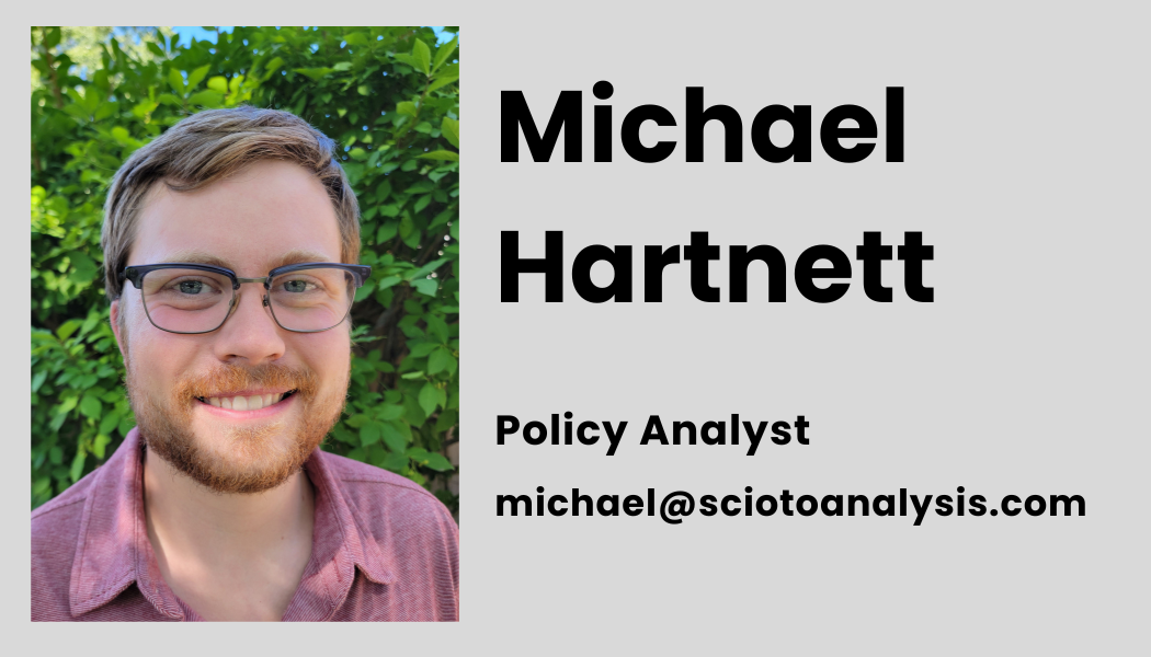
Where the policy analyst ends and the policymaker begins

At the Society for Benefit-Cost Analysis annual conference earlier this month, the lunch keynote on the first day focused on the difficulty of doing good policy analysis in the face of conflicting data. One topic that Sherry Glied, Dean of NYU’s Wagner School of Public Service spoke on was the role of the policy analyst as opposed to the role of the policymaker. This is a topic we talk about a lot at Scioto Analysis and I thought it would be valuable for me to share a little bit about how we think about this important relationship.

Policymaking is entirely about understanding tradeoffs. As an analyst, my goal is to use the best available data to make those tradeoffs clear to policymakers in a way that is honest and accurate. 

It then becomes the role of the policymakers to decide which tradeoffs they want to make. In a well functioning democracy, the policymakers will reflect the view of the people they represent as best they can and allocate whatever scarce resources they have. 

This is where policy analysis and policymaking can sometimes conflict. A policymaker might choose to make a decision that does not maximize efficiency, equity, or effectiveness for some reason. Maybe a policy is very efficient only after we count long-term costs, or perhaps it improves equity concerns but would otherwise be inefficient. 

It can be hard as a policy analyst to accept the fact that always maximizing efficiency is an impossible goal. On one hand, it is impossible because in order to be certain that we were maximizing efficiency we would need to research every possible alternative which would lead to a never ending cycle of research. 

More importantly though, efficiency isn’t always the goal of policymakers. Policymakers have to care about things like elections, political feasibility, and legislative rules.

Often, this separation gets painted as a negative consequence of our political system. “If only the policymakers just did what the research suggests, then we’d have a much better society.” But I don’t necessarily think this is the case. 

For one thing, this separation allows policy analysis to (in theory) operate outside of the political discourse. Of course, there are critical assumptions the analyst has to make that can shape the results quite significantly, but good policy analysis is clear about these assumptions and often tests what happens if they do not hold. 

Once assumptions have been established, applying the best available data and methods should result in analysts coming to the same conclusions. Keeping an arms length away from debates about politics allows policy analysis to maintain its status as a scientific discipline that deals with the truth. 

The other reason this separation is important is because policy analysts are often in the business of predicting the future, which is an inherently difficult proposition. Even the most rigorous analyses can sometimes guess incorrectly about what the future will hold. That doesn’t mean the analysis was bad, just that something unexpected happened. 

Statistics give us the tools to measure uncertainty and incorporate it into our estimates, but at the end of the day most policies only get one chance. It might be a more efficient world if the entire political system was centered around maximizing the expected value of our policies, but it might not. 

Separating policy analysts and policymakers protects the integrity of the policy analysis process. It keeps the focus of the analysis on the process instead of the results. For the most part, as long as the analysis was done correctly, the analyst will continue to be trusted. Conversely, policymaking is a much more outcome focused business. If an expensive program doesn’t work as expected, usually the elected official is going to be on the hook. 

All of this is certainly a glass-half-full take of the dynamics between policy analysts and policymakers. The entire reason Scioto Analysis exists is because we don’t think there is enough good policy analysis happening at the state and local levels of government. 

Good policy analysis should be a much larger part of the way our society functions, we’d all be better off for it. However, it can’t be the entirety of our decision making process. Policymaking and politics still play an important role, and they likely always will. And in a democracy, they probably should.

What is the marginal utility of a dollar?

When I was in high school, I took part in a state government simulation called Buckeye Boys State. High school students come from across the country and take part in a mock state government–passing bills, running cities, operating the state bureaucracy.

I ran for the House of Representatives (after a spectacular failure in the state Senate race) and served in this mock legislative body’s minority party.

While I was serving, one of the majority party members put forth a proposition to institute a “flat tax” for Ohio: a tax rate that was exactly the same for everyone. High schoolers throughout the room nodded. After all, why shouldn’t the tax rate be the same for everybody? You still have to pay a higher amount if you make more money: why should the percentage go up, too?

Being a high school debater, I was always taught to try to debate both sides of an issue. After all, if this issue was so cut and dry, why do we have a graduated tax structure (a tax system where people with more income pay a higher percentage on that income) in the first place?

What I came across was an interesting concept: the marginal value of money. The idea is this: as your income increases, the value of extra income decreases. If a family at the poverty level loses 10% of their income, that will have a much more negative impact on their well-being than a family making five times the federal poverty level.

This plays out in a number of the lenses we use to analyze public policy. From a classical economic standpoint, the idea of the marginal utility of income goes back to 19th century economists. From a poverty or inequality analysis perspective, dollars accrued to low income households are more effective at reducing poverty than dollars accrued to upper-income households.

From a capabilities perspective, basic needs for education and health tend to have marginal utility, too. For instance, the difference between getting no regular health screening and any regular health screening generally improves health more than the difference between getting any regular health screening and the most expensive health screenings. And the difference between no college and going to a low-cost state school is much more vast for future outcomes than the difference between going to a low-cost state school and an ivy league college.

This even plays out in research around subjective well-being. Happiness economist Matthew Killingsworth finds that increases in income correlate with increases in self-reported happiness–but that the increases diminish as income grows. So money does make you more happy, but typically you need a lot more money to get just a little more happiness as you move up the income scale.

So how does this matter to an analyst? My graduate school benefit-cost analysis professor Dan Acland presented a paper at the Society for Benefit-Cost Analysis’s annual conference this month on how to factor this insight into benefit-cost analysis.

His general proposal is to separate impacts of a policy into impacts for lower-income and upper-income people and then adjust dollar values into “income-adjusted values.” In Acland’s model, these can be understood as the value of an impact adjusted for if the beneficiaries were at median income.

In practice, this will make policies that accrue monetary benefits for low income individuals yield higher net present value than they would before adjustment. 

Acland’s proposal is radical, but it seems like a useful way to apply a rigorous equity lens to policies that are likely to have disparate impacts to households across the income spectrum. And we could certainly use better tools to understand the equity impacts of public policy in the United States today.

Ohio economists: extending child work hours will not develop tomorrow's workforce

In a survey released this morning by Scioto Analysis, the majority of economists surveyed thought the proposed extension of hours eligible to be worked by 14 and 15 year olds would not meaningfully help these teenagers develop human capital. Senate Bill 30 would allow these teenagers to work until 9:00 p.m. during the school year, currently they can only work as late as 7:00 p.m. most nights.

Kevin Egan of the University of Toledo writes “the overall limit for hours worked for this group is the same, it just allows later hours to 9 pm. I expect very small to no impact on learning and human capital development, as the only change is allowing the hours of work to be a little later.”

Additionally, the majority of economists surveyed think this proposal might decrease safety for young workers. Jonathan Andreas of Bluffton University, one economist who agrees wrote “... not a big change, but it would increase the number of days that kids are commuting home after dark and the number of hours working after dark and more accidents happen after dark.”

The economists who disagreed pointed to the fact that some teenagers might substitute other risky behavior for later working hours. “14 and 15 year olds are probably safer with employers than other ways they would spend their time,” writes David Brasington of the University of Cincinnati. 

The Ohio Economic Experts Panel is a panel of over 40 Ohio Economists from over 30 Ohio higher educational institutions conducted by Scioto Analysis. The goal of the Ohio Economic Experts Panel is to promote better policy outcomes by providing policymakers, policy influencers, and the public with the informed opinions of Ohio’s leading economists.

Should hybrid cars pay for roads?

The Ohio House of Representatives recently passed a two-year, $12.6 billion transportation budget.

The budget included a number of different provisions, including billions of dollars for pavement and bridges, dollars allocated specifically for economic development projects, and $3 billion for Cincinnati’s Brent Spence Bridge.

One small provision of the bill, however, makes a tweak to the current hybrid car registration process. This change will reduce the registration fee for a plug-in hybrid vehicle from $200 to $100 on Jan. 1, 2024.

Fees for hybrid and electric vehicles have been a bit of a political football over the past few years of Ohio politics. Fiscal conservatives have increased fees hoping to recoup some of the losses to the state from reduced gas tax fees. Environmentalists have decried this policy, saying public policy should be rewarding use of electric and hybrid cars, not discouraging it.

In 2019, Scioto Analysis released a white paper that is pertinent to this conversation. In this paper, we highlight the four major costs of vehicles on the road.

First, there is congestion. The more vehicles on the road, the harder it is to drive and the more time people spend in vehicles driving than at their destination. This exacts a cost on society in the form of time.

Second, there are crashes. More vehicles on the road means more people dying from motor vehicle crashes. This exacts a cost on society in the form of vehicle repair and replacement as well as medical spending and loss of life.

Third, there are emissions. Internal combustion engines emit local emissions that have impacts on local public health and ecosystem health. They also emit carbon, which acts as a greenhouse gas and drives global climate change. These exact costs on society in the form of medical spending, loss of life, and the many dynamic impacts of climate change.

Lastly, more vehicles on the road means more wear and tear on the roads. Since roads are paid for through public spending and are treated as more or less a public good, more vehicles means more costs for taxpayers. This exacts costs on society in the form of more spending on public infrastructure.

Electrification of vehicles (in conjunction with evolution of our energy generation system) can lead to lower emissions. But moving to an electric vehicle will do little for congestion, safety, and infrastructure sustainability.

Gas fees have historically been used as a proxy for infrastructure use. If you drive more, you wear the roads down more. You also buy more gas, which has fees that pay for roads.

The problem the diversification of car fuels presents to this old system of road funding is that now the burden of paying for roads is shifting toward people who have internal combustion engines. This poses concerns for both equity (considering mostly wealthy people own electric cars now) and efficiency (considering those people can now free ride on payments being made by others).

A true 21st-century transportation plan will find a way to implement a vehicle miles traveled fee on all vehicles separate from a gas tax that would capture the cost of emissions. Gas-powered transportation should be more expensive than electric-powered transportation (assuming clean electric generation, which is not really the case today) because of the negative externalities associated with burning of fossil fuels.

Proceeds from fees can be used for rebates for poor drivers or low-income people more broadly, targeted economic development in low-income neighborhoods, or early childhood programs to offset their regressive nature.

We can do transportation policy better in Ohio. And soon enough, we will have to.

This commentary first appeared in the Ohio Capital Journal.

Should we use different discount rates for different projects?

The discount rate is one of the most important considerations of a cost-benefit analysis. It is a critical component that allows us to determine the value we place now on benefits that do not accrue until later. 

Essentially, the discount rate is how we measure uncertainty about the future value of our expected benefits. For example, $100 of benefits today is better than $100 worth of benefits in 50 years because the world in 50 years will likely be very different from the world today. Therefore, the benefits we earn (or costs we incur) tomorrow might not mean as much as benefits earned today.

In order to determine a policy that has benefits 50 years into the future is more efficient than one that has benefits today, we’d need to factor this uncertainty about future benefits into our cost-benefit analysis.

In policy analysis, the selection of the discount rate can dramatically change how we value different proposals. Higher discount rates mean we are less certain about future benefits, and therefore would prefer projects with short-term gains. If the discount rate is too high, we might be short sighted and not plan far enough ahead as a society, valuing present benefits inordinately over those accrued in the future.

Smaller discount rates often make it more likely that future benefits outweigh short term costs. From a policy perspective, this would lead to much more spending on big investment projects. However, if we don’t discount enough, we might be worse off in the short term for projects that might not pan out very well.

In the United States, the base discount rate recommended by Circular A-4 is 7%. The best practice in cost-benefit analysis is to see if your results are sensitive to changes in the discount rate, but for all projects that is the base number to use. For the vast majority of agencies in the cost-benefit analysis world, a single discount rate across projects is preferred.

However, there is one prominent exception to this rule. Analysts in France use variable discount rates depending on the riskiness of the project. For example, imagine we had to choose between investing in a new hospital or in new railroad infrastructure.

Both have massive short term costs and only begin creating benefits after their completion. The main difference is the riskiness of those benefits actually coming to fruition. The hospital will almost always be a useful investment. The “worst case” scenario for the hospital would be if in the future there were no major disasters or pandemics and those hospital beds remained empty. 

Conversely, the railroad infrastructure is much more likely to not realize its benefits. More railroads are important during strong economic times when there are lots of goods that need to be shipped around, but there are always periods of economic downturn. It is much more likely that we will eventually face a difficult time in the economy than we will suddenly not need hospital beds.

Given the intuitive understanding that the discount rate is a tool we have to measure the risk associated with long term benefits, this approach makes a lot of sense. If we can get an idea of how much risk is associated with each type of policy proposal then we would do a better job of efficiently allocating resources. We can do this by allowing for different discount rates between projects. 

There is little consensus among economists about how to choose discount rates for different policies. Because the discount rate can have a significant impact on the results of cost-benefit analysis, it is important that there is a well defined method in place. Allowing analysts to choose discount rates without any framework to back up their choice could lead to severely biased results, and would open the door to potential manipulation.

Currently, the French government adjusts discount rates by looking at price and income elasticities for the goods generated by a policy proposal. This seems to have some strong promise, but in order to fully understand it, more policy analysis needs to be done using it.

Is early childhood education good economic policy?

Last week I attended the Society for Benefit-Cost Analysis’s annual conference in D.C. This was the first time the Society had met in person in four years, having canceled the 2020 conference just weeks before it was scheduled in March of that year.

This year’s conference was a doozy. Presentations ranged on topics from distilling a large evidence base for a topic to factoring the marginal value of money into cost-benefit analysis to variable discount rates due to risk. But the keynote everyone was excited about was given by Nobel Prize-Winning Economist James Heckman.

James Heckman is 78 years old but speaks with the spryness of someone decades younger. Heckman won the prestigious John Bates Clark Medal in 1983 for his work on time series analysis. In 2000, Heckman was awarded the Nobel Prize in Economics for his work overcoming statistical sample-selection problems.

What makes Heckman so compelling for me, though, is the practicality of his insights. Despite much of Heckman’s work seeming to be rooted in esoteric econometric matters, he has become most famous in policy circles for his championing of early childhood education.

In particular, Heckman has analyzed the long-term effects of two famous early childhood programs: the Perry Preschool Project and the Abecedarian Project. 

The Perry Preschool Project was a randomized early childhood program conducted in the 1960s that we now have six decades of data on. The program was offered to low-income African-American children age three and four who were assessed to be at high risk of school failure. Participants in this early childhood program were arrested less before age 40, had higher income, were more likely to graduate from high school, and even had higher IQs later on.

The Abecedarian Project was a similar program conducted in the 1970s in North Carolina. This study was also a randomized controlled trial but took the treatment a step further, offering education to children starting as infants. Participants ended up with better educational outcomes, higher college matriculation, less teen pregnancy, less marijuana abuse, and less depressive symptoms.

Heckman has championed the Perry Preschool model as not just a model for increasing educational, crime, and earnings outcomes for participants, but even for their children. Now that generational data is available on this program that is over half a century old, Heckman argues that early childhood education is a powerful tool for breaking the cycle of intergenerational poverty.

This research is backed up by the research of another giant of the economic policy world and benefit-cost analysis Timothy Bartik. Bartik started doing applied economic analysis focusing on tax incentives and evaluating how their design contributes to improvements in local wages. He was approached by a foundation that was interested in applying his economic development model to early childhood programs.

The worry these funders had was that local leaders would shy away from funding early childhood programs because the children who receive the education would move away and the benefits would not accrue locally. If this were the case, local policymakers would be funding a program that would be building the workforce of other cities.

Bartik’s research found that indeed these benefits would accrue locally. He used results from the Perry Preschool and Abecedarian projects and found that local wage benefits would outweigh the cost of the programs, even factoring in how many children would move away from the local jurisdiction over their lifetime.

Perry Preschool and the Abecedarian Project are only two small-sample studies, but it is not often that we get a randomized controlled trial with accompanying panel data that follows the participants for decades. Only a handful of studies follow a panel of people through their life course like this one and very few are focused on the results of a randomized controlled trial. While there is always more data to collect and evaluation to conduct, the evidence brought forth by economists like Heckman and Bartik suggest early childhood education is indeed a good investment.

A look at the Ohio Opportunity Index

Recently, the Ohio State University released their Ohio Opportunity Index, a report that measures outcomes for residents across the state at the census tract level. Additionally, they released an interactive dashboard that helps visualize the data. 

Here, I take a look at some of the top findings from the dashboard in Franklin county. Which census tracts are doing well, and where can policymakers find ways to improve peoples’ wellbeing. 

Overall Opportunity

In Franklin county, the area with the lowest overall opportunity score was downtown Columbus. Low opportunity extends North of downtown into the South Linden neighborhood. The German Village neighborhood differs from its neighbors by having a relatively high opportunity score relative to the state as a whole. 

Surrounding suburbs like Bexley and Grandview Heights have very high overall opportunity scores. The farther out suburbs also generally have higher overall opportunity when compared to downtown Columbus, though there are some notable exceptions, especially East of downtown.

Education Opportunity

In Franklin county, the general rule of thumb is that the closer to downtown you get the worse the education opportunity is. Poor education opportunities extend in the North in the neighborhoods between I-70 and I-270. To the west, areas of low opportunity are bounded by I-270. 

One major exception to this rule is Bexley, which sits as an island of high education opportunity near downtown Columbus. The surrounding suburbs also once again areas of much higher educational opportunity when compared to downtown.

Employment Opportunity

One major bright spot for Franklin county is how it scores on employment opportunity. Almost the entire county except for a few census tracts near downtown are near the rank near the top of the state. 

Generally speaking, employment opportunity in the state is higher near the major cities. The more rural parts of Ohio often have lower employment opportunity. In particular, the Appalachian region in the Southwestern part of the state scores poorly on this metric. 

Transport Opportunity

For transportation opportunity, we see that most of the city center actually scores better than some of the surrounding suburbs. There is still a noticeable section of low opportunity tucked in the heart of downtown Columbus, but by and large the city has good transportation. 

The suburbs in Franklin county are fairly mixed in their transportation scores. Most of the distant census tracts score poorly, but there are enough good scores mixed in to prevent this from being a discernible trend.

Health Opportunity

Franklin county scores slightly lower on health opportunity than any of the other metrics mentioned above. The main driver behind this is lower scores in the South suburbs. Broadly, we observe the same areas of low opportunity near the city center with the same neighborhood exceptions in German Village and Bexley.

It is not terribly surprising that many of these scores seem to be correlated with one another. Much of this can likely be attributed to local income and poverty rates. Hopefully, the high job opportunity score in the heart of Columbus might mean that some of these other metrics might begin to improve. 

The utility bailout House Bill 6 made both Ohio’s air and politics dirty

With all the drama surrounding the Householder trial for racketeering, it can be easy to forget the bill behind the former Ohio Speaker of the House’s alleged $60 million payoff from First Energy power company.

House Bill 6 had four major impacts. It required power consumers to bail out two massive nuclear power plants in northern Ohio. It also required Ohio ratepayers to bail out two coal plants: one in Ohio, one in Indiana. It reduced energy efficiency standards, requiring Ohio utilities to reduce energy use by 17.5% rather than the previous goal of 22%. Lastly, it reduced Ohio’s renewable portfolio standard, requiring utilities in Ohio to generate just 8.5% of their power from renewables, lowest in the country among states with standards.

I want to focus on the last impact: reducing Ohio’s renewable portfolio standard.

In 2008, Ohio unanimously passed Senate Bill 221, a bill to require 12.5% of Ohio’s energy to be produced from renewable sources. It was an optimistic time for Ohio’s energy transition.

This optimism started to fray in the 2010s. In 2014, a group of state senators led by now-Congressman Troy Balderson pushed through a bill to freeze the standards in place until 2017. Balderson had originally called for a “permanent freeze” but had it changed to temporary after negotiations with the Kasich administration.

In 2019, Householder pulled off what Balderson couldn’t. With HB 6, he reduced the final goal for Ohio’s renewable energy to 8.5% and pushed back its date from 2022 to 2026.

What will this mean for Ohio? Scioto Analysis released a study in 2021 on carbon emission reductions which found that renewable portfolio standards could be as effective as a carbon tax or a cap-and-trade program at reducing carbon emissions in the state. 

We looked at two approaches: a renewable portfolio of 25% by 2026 based on Michigan’s renewable portfolio standard and a renewable portfolio standard of 80% by 2030 and 100% by 2050 based on Maine’s renewable portfolio standard.

We found that both approaches would be effective at reducing carbon emissions in Ohio and would both drive the global cost of these emissions down from over $45 billion a year to under $25 billion a year.

Reducing reliance on coal and natural gas for power would have ancillary benefits as well. Burning of coal releases contaminants into that air that can lead to respiratory illness. Extraction and production of natural gas can have similar impacts as well as lead to a range of other health impacts.

Use of fossil fuels also poses health equity problems for communities. A 2021 study published in Science Advances found racial-ethnic minorities in the United States are exposed to disproportionately high levels of ambient fine particulate air pollution (PM2.5) than white populations, further compounding inequities already experienced between racial groups. Since Black Ohioans already experience poverty at rates nearly three times as high as white Ohioans, this just compounds inequities in the state.

It’s not often that scandal is so closely wedded to policy, but right now Ohio is dealing with this biggest racketeering charge in history, which stemmed from negotiations over its biggest piece of environmental legislation of the century. Let’s hope we can learn from this and find ways to keep both our air and our politics clean.

This commentary first appeared in the Ohio Capital Journal.

How to be a bayesian policy analyst

By and large, humans are pretty bad at understanding probabilities. We live in a world of tangible things and real events which makes it hard to wrap our heads around the abstract concept of randomness. 

Among statisticians, there are two broad philosophies when it comes to thinking about uncertainty: frequentist statistics and bayesian statistics. 

Frequentist statistics assumes that there is some true probability distribution from which we randomly observe some data. For example, imagine we were flipping a coin and trying to determine if it was fair or not. 

A frequentist would design an experiment, and determine a hypothesis test. “I am going to flip the coin 50 times, and I will say the coin is not fair if I get less than 20 or more than 30 heads.”

From this frequentist experiment, we will be able to produce a p-value and a confidence interval. These tell us about the probability of observing our particular set of 50 coin flips, out of the universe of all possible sets of 50 coin flips.

On the other hand, Bayesian statistics relies on our prior knowledge about random variables as the foundation model. These prior assumptions can be the result of historical data or simply the statisticians' judgment.

Take the same coin flipping experiment, we no longer begin by defining a null hypothesis and some criteria to reject it. Instead, we begin with a prior distribution, perhaps assuming the coin is fair, and our goal is to create a “posterior distribution.” In this case, the posterior would be what is the probability the coin is fair.

Assume now that we ran our experiment and flipped 21 heads in 50 tries. In this case, the frequentist would say “We fail to reject the null hypothesis and can not conclude whether or not the coin is fair.” The Bayesian would instead find the posterior distribution, and be able to make a statement about the probability the coin is fair.

In short, the frequentist will never calculate the probability of a hypothesis being true. They will either reject it or fail to reject it. A Bayesian statistician will always begin with a prior guess about whether a hypothesis is true, and update that prior guess as they observe new information.

I personally find Bayesian thinking to be a much more satisfying way to conceptualize uncertainty. We all carry around some prior knowledge about how random things should play out, and as we observe new information we update those priors.

However, one thing to realize about intentionally thinking like a Bayesian is that it is often slow to incorporate new and dramatically different pieces of information. This can be good when the dramatically different information is an outlier that we don’t want to have completely determine how we think, but our priors can be slow to recognize when things do change dramatically.

In practice, I still mostly use frequentist statistics as part of my analysis. In practice, Bayesian analysis is often sensitive to the construction of the prior distribution and it is not always useful to a policy maker when the result of some analysis still has probability baked in.

Still, Bayesian statistics reminds us that we live in a world where things are uncertain. Especially in policy analysis, where we often try to predict future outcomes, it is important to remember that there is uncertainty and unlikely outcomes do not necessarily mean our predictions were wrong.

Ohio economists pessimistic about proposed school voucher program

In a survey of Ohio economists released this morning by Scioto Analysis, the majority of respondents disagreed or were uncertain that the proposed increase of Ohio’s private school voucher program would increase standardized test scores for Ohio’s students. “There are a lot of complex dynamics (some students may see higher scores but others may see lower scores) but almost certainly there will not be a significant effect on the average test scores in the state,” said Dr. Curtis Reynolds of Kent State. 

When asked if the proposed voucher increase would lower the quality of Ohio’s public schools, 11 economists agreed, four disagreed, and seven were uncertain. Dr. Kay Strong, who strongly agreed, said “the proposed upper threshold of $111,000 earning for a family of four assuming two are children will exacerbate the privilege of high income families at the cost of lower quality education from reduced public spending on traditional public school.” 

Since we surveyed the panel, the Ohio senate has introduced Senate Bill 11 which would create universal school vouchers.

The Ohio Economic Experts Panel is a panel of over 40 Ohio Economists from over 30 Ohio higher educational institutions conducted by Scioto Analysis. The goal of the Ohio Economic Experts Panel is to promote better policy outcomes by providing policymakers, policy influencers, and the public with the informed opinions of Ohio’s leading economists.