How to talk about statistics to non-statisticians

The final required class I took in grad school was called “Statistical Consulting,” and unlike every other course I took I did almost no actual statistics in it. Instead, this course predominantly focused on how to take all of the fancy methods and advanced concepts I had learned over the last two years and communicate the results to people without a background in statistics. 

As a policy analyst, I find myself communicating with non-statisticians more often than in school. This is an exciting opportunity to share the statistical tools I have with an audience that can meaningfully apply my results. These are some of the things I learned that have helped me better explain complicated concepts to a less technical audience.

Ask your audience for their statistical background

During my first ever consulting project as a grad student, I spent about 10 minutes of my first meeting going over the pros and cons of using a time-series approach with the client before they had the opportunity to ask me what a time-series model was. This is not to say that the discussion on the pros and cons of the time series approach was wrong or that the client didn’t need to be included in that conversation, but rather that had I known my client’s background I would have approached that discussion differently.

In this particular case, my client wasn’t interested in the statistical differences between the models I was proposing, but rather what the practical differences would be in the final report. After resetting, we were able to have a much more productive discussion that was tailored to his level of understanding. 

Use visuals when possible

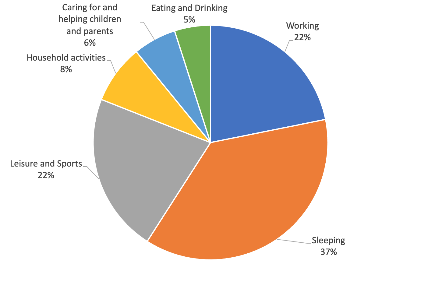
Good data visualizations can communicate a complicated idea almost instantly, especially when paired with a clear written description of the main takeaways. However, it is important to not get carried away with visualizations. 

One common mistake is visualizing every possible part of an analysis. Visuals are great for highlighting the most important parts of a report. Highlighting everything might make it harder to find the most important pieces of information. 

Another consideration to have is when to use a graph or a table to visualize data. A general rule of thumb is to use tables when the specific value of a result is important and graphs when the broader trend is important. 

Provide context

Statistics never exist in a vacuum, and it is important to provide context in order to make your results more useful. Being upfront about what data or methods you used, what the strengths or weaknesses of your approach were, these are the sort of non-result pieces of information that help people understand the full picture of an analysis. 

Be honest

There are a whole lot of approaches we can use when analyzing data, and some of these approaches might allow for different interpretations of the results. Statistics sometimes gets viewed as a scientific and objective way to examine the world around us (which it largely is), but the perspective of the analyst has a lot of weight in determining the final message. 

Always make sure you are being clear about the assumptions your models make, and the limitations of your results. It goes without saying that intentionally misleading charts or excluding critical information has no place in any respectable analysis.

How do Americans spend their free time?

A central theory of labor economics covered in most introductory microeconomics courses is that of the “labor/leisure tradeoff.” This is the concept that workers have time they can spend working and time they can spend doing other things and that they will try to maximize their “utility” by achieving the optimal mix between labor and leisure.

Below is a visualization of the concept. You can plot a wage on a chart like this as a line that runs from the top left to the bottom right and a worker will choose how much to work based on where their wage line intersects the “indifference curve” (the blue lines) that is furthest out. An “indifference curve” represents all the points as which a worker would be “indifferent” to a different mixture between income and leisure. 

So a worker is just as happy at being at point A or point B who has the indifference curve IC1, though at point A she has more income and less leisure and point B she has more leisure and less income. Any point to the northeast of IC1 is preferable to any point on IC1 because it means more income and more leisure, less leisure compensated by much more income, or less income compensated by much more leisure.

This is of course a simplification. There are structural frictions in the labor market that can limit a worker from achieving the appropriate mix of labor and “leisure” that she desires. But empirically we do see this phenomenon playing out, with price increases like taxes leading to reductions in labor time in favor of “leisure” time. What I’m more interested in talking about here is something else: what we define as “leisure.”

“Leisure” time is defined by this model as time a worker spends doing something other than generating income. But is all of this rightly understood as “leisurely” activity?

One place we can look to find an answer to this question is the American Time Use Survey. The American Time Use Survey is a nationally representative survey conducted by the Census Bureau to determine how, where, and with whom Americans spend their time. It is the only federal survey providing data on the full range of non-market activities, from childcare to volunteering.

Looking at an overview of how Americans spend their time, the picture of “leisure time” gets a little more complex.

According to 2021 results, Americans spend about 22% of their time on average at work. They spend about 37% of their time on sleeping, 22% of their time on leisure and sports, 8% of their time on household activities (including travel), 6% of their time on care for children and parents, and about 5% of their time on eating and drinking.

So if we look at these results, we find that 42% of total time (54% of what the labor/leisure model calls “leisure time”) is spent on eating and sleeping, activities most people would deem essential to survival. Yes, there is a leisure component to eating and sleeping, but many people’s experience with food and sleep in the United States would not necessarily be called “leisurely.”

Another 14% of total time (18% of “leisure time”) is spent on household activities and caring for family members. This is what many would consider “non-market economic activity”--dollars aren’t changing hands, but they certainly could if these activities were outsourced from the household to a cleaning service, child care agency, or long-term care facility.

This only leaves 22% of total time, or 28% of time not worked, as time for “leisure and sports.” So only about a quarter of what we call “leisure time” is truly spent doing things we consider “leisure.”

When I was in graduate school, our economics professor eschewed the use of the phrase “leisure time” for the phrase “non-market time.” I think this is probably a better way to treat this time we spend sleeping, eating, taking care of family, caring for the house, and on leisure and exercise.

How can we prevent the next East Palestine?

Ohio is in the national news again, this time around a tragedy that sits at the crossroads of transportation, environmental policy, and public health. The high-profile train derailment at East Palestine, Ohio started as a shocking evacuation. It has since grown into an international story about the impacts of the derailment on the environment and the health of people near and far from the disaster.

In the wake of this event, policymakers have been asking for answers. Much of the public policy focus has zeroed in on a rule-making saga that has played out over the past few years at the federal level.

A couple of high-profile derailments in 2013 and 2014 led the Obama administration to issue a rule requiring electronic brakes for high-hazard, flammable trains in 2015. Three years later, the Trump administration repealed the rule.

Some believe this rule could have prevented the East Palestine derailment. Steven Ditmeyer, a former senior official at the Federal Railroad Administration, said “applying the [electronic] brakes would have stopped everything very quickly.”

So is that it: open and shut case, just need to require electronic braking systems, dust our hands off and go home?

Let’s not move so fast. What is really causing severe derailments in the United States? And is there something we can do about it?

The former question was asked by a researcher at the Department of Civil and Environmental Engineering at Rutgers and a team of international engineers analyzing train derailments in the U.S. The engineers analyzed over 20 years of freight derailment data in the United States to determine what was driving freight derailments across the country.

Let’s use these results to identify the root causes of train derailment. Four of the top ten causes for freight train derailment these engineers found were track-related factors. These included wide gauges, buckled tracks, track geometry, and most importantly broken rails or welds. 

Broken rails and welds led to not only the most severe derailments, but also was by far the most frequent cause of derailment. All in all, track-related factors made up three of the four factors that led to the most severe derailments. 

Only two of these top ten factors were related to rolling stock (the trains and cars themselves). These two factors were broken wheels, which were less common but led to more severe derailments, and bearing failure, which were more common but led to less severe derailments. Braking failure was notably absent from this top ten list.

While better brakes could have some impact on train derailments, if we can learn anything from history, it is that train derailments are most often directly caused by the most obvious factors: shoddy tracks and dilapidated trains.

Investment in fixing broken rails and welds, buckled tracks, track geometry, and wide gauges could be an effective approach to reducing freight train derailments. This could be done through grants, loans, regulation, or a combination of the three. 

Other areas of improvement are in ensuring cars are tip-top by maintaining wheels and bearings and making sure tracks are free of obstruction. These approaches could also be achieved through grants, loans, and regulation.

These strategies for reducing train derailment are not as sexy as electronic braking, but could be just as effective. Policymakers should use this as an opportunity to let the evidence guide better policy and prevent future disasters from occurring.

This commentary first appeared in the Ohio Capital Journal.

5 charts to better understand poverty in Franklin county

Poverty is a perennial topic in public policy. In order to make good policy decisions about poverty, we need to understand what poverty is and what it means to the people that experience it. 

Since Scioto Analysis is headquartered in Franklin County, I thought it would be valuable to share some information about poverty in a U.S. urban area using Franklin County as a case study. Here are five charts that help contextualize the current state of poverty in Franklin county. 

Poverty rate over time

The past decade of poverty trends in Franklin County has been defined by recovery from the Great Recession. The highest reported poverty rate in two decades before the 2008 recession according to the St Louis Federal Reserve was 16.4%, but county poverty rates topped out at nearly 19% in the years after the Great Recession. It took over 10 years for poverty to return to pre-recession levels. 

Another takeaway from this chart is that the county did not take the same hit during the COVID-19 recession as it did during the 2008 recession. Part of this was due to temporary assistance issued during the pandemic, which was successful in keeping poverty rates down. Programs like the expanded child tax credit were also crucial in keeping people afloat, but are post-tax income so not included in official poverty measure calculations. This means something more was at work during the COVID recession. 

Poverty rates by race

There are significant differences in poverty rates by race in Franklin county. Black and Native American residents of Franklin County are more than twice as likely to be in poverty as white residents. Hispanic/Latino residents are nearly twice as likely to be in poverty as white residents as well. White and Asian residents are the two groups that experience poverty at lower rates than the county as a whole. 

Total poverty by race

Despite the fact that white residents experience poverty at the lowest rate of any racial group in Franklin county, the majority of people in poverty in the county are white. This is because white non-hispanics make up 61% of the total population according to the 2020 census. 

The difference between absolute poverty statistics and relative poverty statistics demonstrate why it is important to look at all of the context when talking about poverty. They seemingly tell different stories about what poverty is like in Franklin county, but in truth both are needed to understand the complete picture. While white residents of Franklin County tend to be less poor than Black and Hispanic residents, the sheer number of white residents of the county means that most people who are poor in the county are white.

Employment and poverty

Unsurprisingly, people who are employed experience less poverty than those who are unemployed. However, when talking about unemployment, we often overlook the problem of underemployment. The official unemployment rate counts underemployed people as employed, meaning that we sometimes overestimate the strength of the job market when we lean on that measure. 

This graph shows the importance of underemployment on poverty. There is a massive gap in the poverty rate between people who worked full time and those who were unemployed, but importantly the part-time/part-year workers experience poverty at a rate much closer to the unemployed group. This demonstrates that not all jobs are equal, and if we want to have some impact on poverty through the labor market we need to make sure that people have enough quality employment. 

Education and poverty rates

In Franklin county, there is a strong positive correlation between education and poverty rates. An individual without a high school diploma is almost twice as likely to be in poverty than someone with a high school diploma, and seven times more likely to be in poverty than someone with a bachelor’s degree.  

Charts like this suggest potential policy paths for alleviating poverty. Presumably, if we were able to increase the rate at which people finished high school or made equivalents easier to access, we could make more people less likely to experience poverty. We also have insights on how race, employment, and long-term trends impact poverty.

What is Monte Carlo Simulation?

As a statistician, I tend to be inherently skeptical anytime I see a single number reported as a prediction for the outcome of a policy proposal. Point estimates are certainly useful pieces of information, but I want to know how likely these predictions are to come true. What is the range of possible outcomes?

In policy analysis, it sometimes seems impossible to certainly tell what the range of possible outcomes might be. What if one input in our predictive model is higher than we think, but another is lower than we think? What if there are so many inputs that it would be practically impossible to test for all of the different possible outcomes? 

It is times like these when we can turn to Monte Carlo simulations to estimate our variance. From Scioto’s Ohio Handbook for Cost Benefit Analysis: “The essence of Monte Carlo simulation is to generate a large number of possible outcomes by varying all the assumptions in the analysis.” By changing all of the inputs at once over thousands of trials, we can more accurately measure the uncertainty in our predictions. 

At their core, all statistical models are essentially just mathematical equations. Imagine we are considering building a new public swimming pool and want to conduct a cost-benefit analysis. In one model, the costs would be the construction and annual maintenance costs, and the benefits would be the average benefit per person multiplied by the number of people that we expect to use the pool. 

Benefit per Person x Expected Visitors - Construction Cost - Annual Maintenance = Net Benefits

The four inputs to this model are not fixed values, but instead are random variables. We can use observed data to create sensible estimates for these random variables, but at their core they are not deterministic. 

We can define a random variable by its probability distribution. A probability distribution conveys two critical pieces of information: what all possible outcomes are and how likely those outcomes are. Once we have real data, we can say that we have an observation or a realization of a random variable. Observations and realizations are associated with a random variable and a probability distribution, but they are not random themselves. 

Let’s apply this to our swimming pool example. To estimate the number of visitors our pool will have, we can collect data about the number of visitors other public pools have. To create a point estimate, we might take the average value of our observations and plug it into our formula. Repeat that process with the other three inputs and you have a basic cost benefit analysis.

However, if we assume that the number of visitors to public pools are all observations of the same random variable, then we can make some claim about the distribution of that random variable. An in-depth knowledge of statistics is needed to make and verify these distributional assumptions, but the point is that we are defining all the possible outcomes and how likely those outcomes are.

With the probability distribution defined, we can use statistical software to generate thousands of observations that all follow the same distribution. This gives us thousands of inputs into our equation and thousands of different results, meaning we can now analyze the range of possible outcomes. 

Monte Carlo simulation really begins to shine once we start defining the probability distributions for all the random variables in our equation. It helps at this step to think of the Monte Carlo simulation as happening in rounds.

In a single round of simulation, we generate an observation for each of our four random variables from their respective probability distributions. One round might have above-average values for the number of visitors and the benefit per visitor but below-average values for the cost variables, leading to well-above-average net benefits. Repeating this for a few thousand rounds will allow us to accurately see the range of possible outcomes and more importantly the likelihood of each potential outcome. 

These simulations often involve a lot of assumptions about the distributions of random variables. Understanding and checking these assumptions is required in order to generate meaningful results. 

Monte Carlo simulation is a powerful tool for analysts to use. It goes beyond just offering a single estimate for a prediction, and provides deeper insight into the likely range of outcomes. If you have the time and the statistical background to perform a Monte Carlo simulation, doing so can dramatically improve the quality of your estimates. 

How do I conduct sensitivity analysis?

When making an estimate of a cost, economic benefit, or some other important policy impact, a policy analyst is carrying out a very difficult task. She is trying to put numbers to things that we often don’t see as quantifiable. Inevitably, any analysis will lean on a range of assumptions in order to get from abstract idea to a number. 

But what happens when we change these assumptions? And what happens if the empirical evidence we use is a little bit off from reality? This is where the policy analyst employs the important tool of sensitivity analysis.

Sensitivity Analysis is the process of estimating how assumptions included in an analysis impact the uncertainty around the findings of the analysis. By conducting sensitivity analysis, we can get an idea of how precise our findings are. We can also report these findings as a range so we don’t oversell the precision of our findings.

But how do we conduct sensitivity analysis? There are a few different ways to do this, but the most common approaches are what we call “partial sensitivity analysis,” “worst- and best-case analysis,” “breakeven analysis,” and “Monte Carlo Simulation.” Below are some explanations of the methods for conducting sensitivity analysis as laid out in the Ohio Handbook of Cost-Benefit Analysis.

Partial Sensitivity Analysis

Partial sensitivity analysis is in some ways the most basic of sensitivity analysis techniques. This technique is carried out by taking one key input and varying it to see how it impacts the results of the study. By showing how one factor impacts the outcome of a study, a policymaker can understand the risks involved in relation to a key factor. 

An example is an input like the “value of a statistical life,” a valuation that has a range of different values depending on what agency is carrying out the analysis. In a study that includes an important input with varying valuations like the value of a statistical life, showing the net present value of the program under different assumptions for the value of a statistical life gives an insight into the variability of the results.

Worst- and Best-Case Analysis

Let’s move on from varying one input to varying multiple inputs. Sometimes when we conduct a cost-benefit analysis or another policy analysis, we may come up with a result that is very optimistic or very pessimistic. In this situation, we can conduct sensitivity analysis to test how reliant our results are on our assumptions.

To carry out this form of a sensitivity analysis, an analyst takes all the inputs and sets them to the most optimistic or pessimistic reasonable assumptions. This allows her to communicate to a policymaker what the policy’s outcomes would look like if all her assumptions are pessimistic and what they would look like if all her assumptions were optimistic. This process also allows her to test her assumptions and see if changing them impacts the ultimate findings of the analysis, determining if it has net costs or benefits under all circumstances or if it ends up above or below water depending on assumptions.

Breakeven Analysis

Some analyses are fixated particularly on finding if a policy has a positive net present value or a benefit-cost ratio above one. In these situations, it is useful to see how much assumptions need to change in order to see when benefits and costs “break even.”

Breakeven analysis is the process of varying assumptions to see where costs would equal benefits. This gives policymakers an understanding of how much the assumptions need to vary from their expectation for the policy’s benefits to exceed costs.This can be modified to broader policy analytic techniques if an approach is created to measure impact against each other: see what needs to be changed in order for two alternatives to be basically the same from an analytic perspective.

One way breakeven analysis can be useful is if the results are particularly robust. For instance, if a policy has a positive net present value unless the average wage for people carrying out the program exceeds $1 million per year, then that would suggest confidence that the net present value of the program is indeed positive.

Monte Carlo Simulation

Sometimes called the “gold standard of sensitivity analysis,” Monte Carlo Simulation is a more complex sensitivity analysis technique that requires data analysis software. The essence of a Monte Carlo simulation is to generate a large number of possible outcomes by varying all the assumptions in the analysis. Using these outcomes, confidence intervals for cost-benefit outcomes can be estimated. Advanced Microsoft Excel users can execute a Monte Carlo simulation with a little bit of help from Google.

Even conducting a simple partial sensitivity analysis can provide useful insights for a policymaker. The point of sensitivity analysis is to estimate precision of estimates, and using any of the above techniques makes an analysis more complete.

DeWine child tax deduction leaves poor families out

At his “state of the state” address on Tuesday, Ohio Gov. Mike DeWine put forth a unique proposal to the Ohio legislature — to enact a $2,500 per child state tax deduction.

When I first saw this, I was excited! The 2021 federal child tax credit expansion lifted over 2 million children out of poverty. After Joe Manchin torpedoed efforts to preserve the tax credit, a number of states moved to create state versions of the effective anti-poverty program. Could Ohio become the thirteenth state to enact a child tax credit?

But then I took a look closer — wait, this wasn’t a state tax credit that DeWine proposed, but a tax deduction.

How a credit works is that you get back money that you owe, sometimes in excess of what you owe. So a $2,500 tax credit would put $2,500 in the pocket of a taxpayer.

A deduction just means that you can subtract that amount from your income to calculate your taxes. So if you make $50,000 in a year and you subtract $2,500 from that, you pay taxes on $47,500 in income. With Ohio’s tax at that bracket of 3.226%, that means you’d save about 80 bucks.

A problem with a tax deduction from an equity standpoint is that they help out wealthy people more than low-income people. This is because the higher your income gets, the more you have to pay in income tax. So those deductions help wealthy families more than low-income families.

What does this look like in practice? Well, let’s look at some examples of how this could shake out for families. 

Ashley Smith is a single mother of two from Jacksontown, Ohio, a small town northeast of Buckeye Lake. She makes an average amount for Jacksontown: a little over $24,000 a year. She would save zero dollars from the proposed child tax deduction.

Jessica Miller is a single mother of two from Dayton. She makes an average amount for a family in Dayton: a little over $43,000 a year. She would save a little under $140 with the proposed child tax deduction.

Amanda Johnson is a single mother of two from Chillicothe. She makes an average amount for a family in Chillicothe: a little over $66,000 a year. She would save a little over $160 with the proposed child tax deduction.

Sarah Brown is a single mother of two from Centerville, Ohio, a suburb of Dayton. She makes an average amount for a family in Centerville, a little over $100,000 a year.  She would save a little over $180 with the proposed child tax deduction.

Brittany Williams is a single mother of two from New Albany. She makes an average amount for a family in New Albany, nearly $208,000 a year. She would save nearly $200 with the proposed child tax deduction.

So Brittany, supporting a family on over $200,000, will receive a $200 benefit from the child tax deduction. Meanwhile, Ashley, supporting a family on $24,000, will receive nothing. Nearly all families in poverty will receive nothing from this benefit, while middle- and upper-income households will receive $70 to $100 per child, with benefits higher for families in higher tax brackets.

If the DeWine Administration wanted to help children in poor families, it could create a better system by providing a credit per child. The administration could even create an income cutoff to keep costs low by targeting benefits toward lower-income households. The current proposal, on the other hand, excludes the families that need help the most while giving the largest breaks to the most well-off Ohio families.

This commentary first appeared in the Ohio Capital Journal.

Two transportation policies that would change how we travel

Households in the United States spend a lot of money on transportation. According to the bureau of transportation statistics, transportation is the second largest category of household spending behind housing–higher than out-of-pocket medical spending, apparel and services, and food. Additionally, transportation is the largest source of greenhouse gas emissions according to the EPA.

For those of us that are always looking for inefficiencies in society to try and improve, these are two pretty significant red flags. Policymakers tend to agree, and often we look to public transportation as a way of improving economic and environmental conditions.

The thought process is fairly straightforward. If fewer people drive their own cars and instead substitute shared transportation into their lives, we can cut back on costs and reduce emissions. 

Broadly speaking, this is a question of a market with an externality and trying to figure out what the best way to correct it is. In situations like this, the two most straightforward policy levers we have to pull are to subsidize public transportation and tax private transportation. Both in theory should make public transportation more appealing to consumers. 

In practice, we most frequently see a tax on private transportation via a tax on gasoline while subsidies on transportation come in all shapes and sizes. These policies present a very interesting case study to talk about efficiency and equity in the context of externalities, so let’s examine two of the most bold proposals that some governments have adopted. 

Vehicle miles traveled (VMT) tax

A vehicle miles traveled (VMT) tax levies taxes based on the number of miles driven in a year. The VMT tax is an alternative to the gas tax that ignores differences in gas consumption between cars. Because wealthier individuals often have better access to high gas-mileage or electric cars, this prevents the tax from being as regressive. It also helps efficiently price the cost of wear and tear on roads, one of the main reasons car use is taxes in the first place.

In theory, a VMT tax would reduce the number of miles traveled in cars by making those miles marginally more expensive. All else equal, we would expect this lost car travel to be replaced by public transportation, carpooling, walking, biking, or reducing numbers of trips. 

One important equity consideration around the institution of a vehicle miles traveled tax is that many people are unable to substitute public transportation because the current infrastructure doesn’t meet their needs. You might think of someone who has to work a night shift after buses stop running.

Another equity consideration is that the number of miles traveled in a year by an individual does not typically increase proportionally with income. So low-income people would still spend a larger proportion of their income on vehicle miles traveled fees than upper-income people. For this reason, a vehicle miles traveled fee would still be regressive, though not as regressive as a gasoline tax.

From a pollution-reduction perspective, this probably would not be as effective at reducing pollution as a gas tax. In fact, if enough people substituted away from electric cars to public buses with gas engines, it could actually worsen pollution. Carbon or other pollution taxes could supplement a vehicle miles traveled fee in order to efficiently price these externalities.

The most interesting question about a VMT is how extra tax revenue would be spent. This is probably the most important question that would determine whether or not this policy would be efficient. After paying for roads, would money be used to upgrade public transportation, to fund other environmental projects, or maybe as a rebate to low income individuals? These options would have different efficiency and equity implications.

Free public transportation 

In five months, Washington D.C. will become the largest city in the country to completely eliminate its bus fees. Other cities like Olympia, Washington and Kansas City, Missouri have already done so. 

This type of policy is becoming increasingly popular due to the argument that it helps low-income riders. The goal of free public transportation is to increase mobility for people who don’t have access to other transportation and to encourage people who do have access to other transportation to instead use public transportation when possible.

In theory, by reducing the price of public transportation people on the margins would begin to choose it over driving their car. In practice, for there to be much of an impact there would likely have to be an expansion of public transportation infrastructure to match its increasing demand and to make sure that it is far-reaching enough to allow everyone to ride. 

From an equity perspective, the program is targeted at lower income individuals. Currently, public transportation is a less expensive way to get around so by making it even less expensive, lower income people will have more discretion with their income. The extent to which it fulfills this goal, however, is up for debate. Many low-income people in a number of categories have subsidized bus passes provided through other public programs. Eliminating bus fares may fill some gaps, but it might not have the equity impact its boosters hope for.

Eliminating fares also targets benefits narrowly on bus riders. Low income people who walk, bike, or use other forms of transportation receive no benefits under this scheme. A vehicle miles traveled fee used to finance a low-income tax credit can theoretically help more low-income people and reduce single-occupancy driving more efficiently and equitably than eliminating bus fees.

—

How state and local governments choose to handle their transportation policy will depend on local factors. If a city already has a robust public transportation infrastructure, then making it free through some sort of progressive tax could reduce equity and pollution. 

If there would have to be a big capital investment to make free public transportation equitable and efficient, then maybe those resources could be better spent on some other poverty reduction or environmental project. Either way, by understanding the potential outcomes of certain policies, policymakers can make the best decision for their constituents with the resources they have.

Which discount rate should I use?

One textbook on cost-benefit analysis says that discounting is not controversial in cost-benefit analysis, but that the rate at which we should discount is. While there are still some fringe voices among cost-benefit researchers who argue for a 0% discount rate, the point is well-taken that most agree discounting is necessary. The point is also well-taken that researchers have not coalesced around a “right” rate to discount at.

Part of this is the nature of the discount rate. The purpose of discounting in cost-benefit analysis is to capture differences in time preference for income for society. If you were offered $100 today or $100 in a year, you’d probably take $100 today. You would need to be offered $103, $105, or maybe even $111 in a year for it to be worth it for you to hold out. Because of uncertainty about the future, a certain amount of income today is widely agreed to be preferable to income later, all else being equal.

A discount rate is ultimately supposed to be about adjusting for how much society prefers current income to future income. This is a hard thing to account for and depends on which society we’re talking about, how they think about income, and the quality of the income (the latter of which can vary significantly in cost-benefit analysis due to the range of outcomes that are monetized).

So if we are going to discount future costs and benefits in a cost-benefit analysis, how do we go about choosing the correct discount rate? Despite the controversy over which discount rate to choose, analysts have coalesced around a few specific recommendations.

3% Discount Rate - The “Consumption Rate”

If you put a gun to my head and asked me what the best discount rate was for any given cost-benefit analysis, I’d have to turn to the 3% discount rate. In a 2021 Resources for the Future issue brief, researchers Qingran Li and William A. Pizer refer to this discount rate as the “consumption rate.”

Li and Pizer say that the 3% discount rate comes from the after-tax earnings on investments. The logic here is that households (who they say are considered the “ultimate authority on ‘welfare value’”) will not favor government policies that yield lower returns than they could receive in the private market.

The 3% discount rate is the rate I have generally seen most and is favored by many because of its focus specifically on time preference and its adjustment downward from the 7% figure due to taxes being included. But don’t count 7% out yet.

7% Discount Rate - The “Investment Rate”

While 3% is the rate I tend to see, it only holds a slight edge over the 7% discount rate, which is based on the average long-term rate of return on a mix of corporate and noncorporate assets. This is the rate of return before taxes, but is still generally considered as a leading discount rate for conducting cost-benefit analysis.

The federal Circular A-94 guidance for discount rates for federal agencies endorses a 7 percent rate for the above reasons, though suggests that higher rates should be used in circumstances where purely business income will be at stake for example since costs will likely be higher due to business’s steeper time sensitivity.

11% - The Developing CountRy Rate

A 2015 technical note from the Inter-American Development Bank says that “In general, developed countries tend to apply lower rates (3-7%) than developing countries (8-15%), although in most cases these rates have been reduced in recent years.” Discount rates are just as controversial in developing countries as they are in developed countries, but traditionally have tended to land around 11%.

More recent reports have recommended lower discount rates in developing country contexts. These are often in light of evaluating the costs and benefits of interventions to mitigate climate change, which tend to front load costs in favor of generating long-term benefits. But there is another way to tackle this problem.

Variable Rate - Accounting for Future Generations

A common approach to dealing with the problem of costs and benefits incurred far in the future is to adopt a variable discount rate, or a discount rate that changes over time. An argument in favor of this approach is that applying a steady discount rate generations into the future privileges the time preference of people in the present over those in the future.

This approach is endorsed by the UK Green Book, the official guidance document from the United Kingdom’s Treasury on how to conduct cost-benefit analysis and other economic analysis. The Green Book recommends a 3.5% discount rate that then declines over the long term.

Sensitivity Analysis

Because of the range of different possible discount rates, my recommendation is to incorporate discounting into your sensitivity analysis. Conduct a partial sensitivity analysis of 3% and 7% discount rates to see how using alternate discount rates impact your results. If costs fall on business earnings, try higher rates to see what happens. Then vary sensitivity analysis in a Monte Carlo simulation to see what range of impacts are possible under different discount rates.

We may not have one discount rate in cost-benefit analysis, but we certainly know enough to try some out and see what they tell us about the policy we are analyzing.

Majority of Ohio economists think "right-to-work" law would deepen inequality

In a survey released this morning by Scioto Analysis, 13 of 22 economists agreed that a “right-to-work” law would increase inequality in the state. Economists who agreed pointed out that right-to-work laws would likely decrease union membership and therefore lower union bargaining power. In theory, this would lead to lower wages for union members, and higher profits for their employers.

On questions of economic growth and employment, economists were evenly split about the impacts of right-to-work laws. In comments, some economists said making union membership non-mandatory could increase employment in some sectors. Others stated this effect might be counteracted by lower wages and slower economic growth. 

One economist points out that states with right-to-work laws don’t experience different economic growth compared to other states, meaning employment effects could be offset by other economic effects. Another mentions that the academic literature on the subject fails to reach a consensus about impacts. 

The Ohio Economic Experts Panel is a panel of over 40 Ohio Economists from over 30 Ohio higher educational institutions conducted by Scioto Analysis. The goal of the Ohio Economic Experts Panel is to promote better policy outcomes by providing policymakers, policy influencers, and the public with the informed opinions of Ohio’s leading economists.