How can we measure poverty better in 2023?

The way we measure poverty is not the best way to do it.

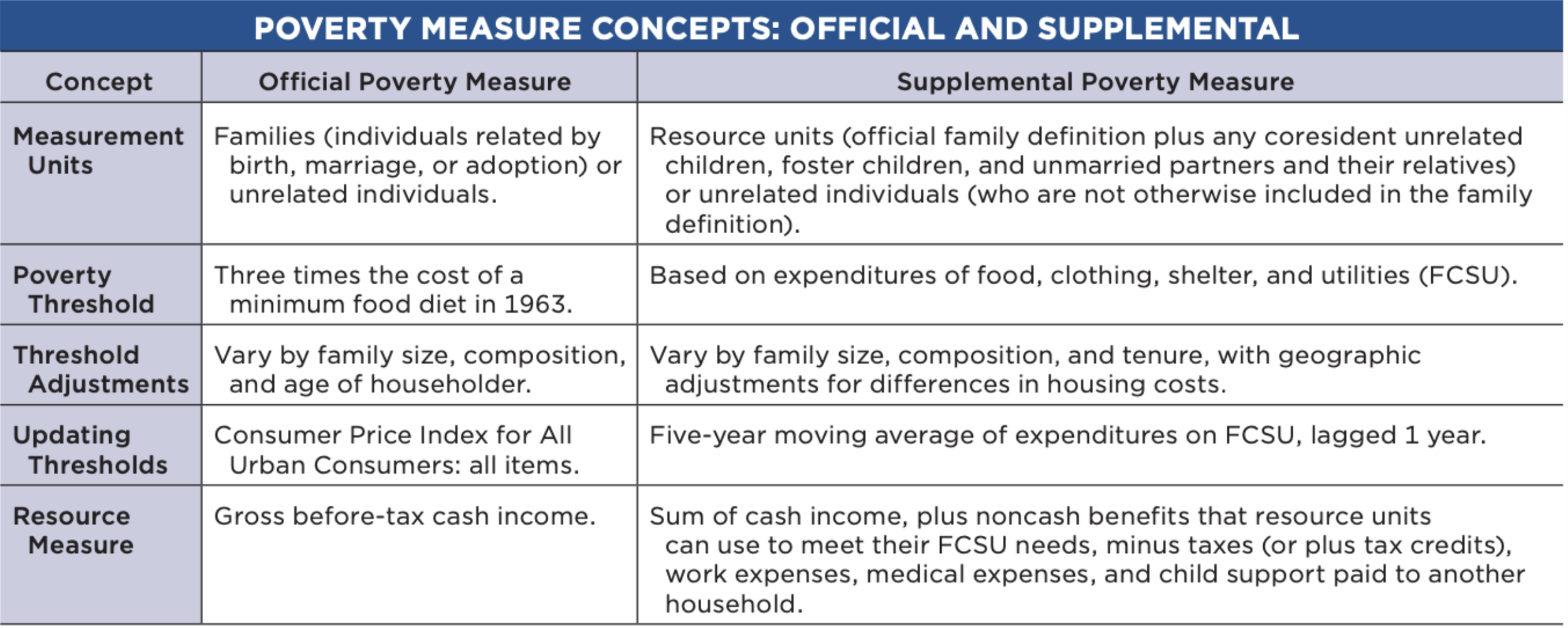
The current poverty measure–known as the “Official Poverty Measure”--was originally developed by economist Mollie Orshansky during the War on Poverty in the 1960s. At the time, the average family spent about a third of their income on food. Orshansky then surmised that a family that had three times the income necessary to pay for a “thrifty food plan” would have the resources necessary to survive. Thus, the official poverty measure was born.

Since then, the economy has changed. Due to advances in agricultural technology, the average family now spends about one-eighth of their income on food. Meanwhile, essentials like health care and housing have gone up in price over time.

Due to these changes in the economy, economists have proposed an update to the official poverty measure. This was first put forth in a 1995 National Academies study to modernize the U.S. poverty measure. The proposal put forth a number of recommendations to modernize poverty measurement in the U.S., but sat on a shelf for over a decade before being implemented.

In the late 00s, New York City calculated the New York Poverty Measure, a new measure of poverty based on the recommendations from the National Academies. Soon after, the Census Bureau calculated the first Supplemental Poverty Measure, a new measure for the United States that incorporates the recommendations of the National Academies study into a new national poverty measure.

The findings of the Supplemental Poverty Measure were a little surprising. Overall, the measure found a nationwide poverty rate very close to the official poverty measure. The real departure, though, comes when the data is disaggregated. 

For instance, child poverty is lower and elder poverty is higher in the Supplemental Poverty Measure than in the Official Poverty Measure. This is because the Supplemental Poverty Measure counts a lot of benefits programs that help families with children as income that the Official Poverty does not. It also subtracts the cost of medical out of pocket expenses from family income, which makes elderly people look poorer than the Official Poverty Measure. 

The Supplemental Poverty Measure also has big impacts on regional poverty. Because it includes a cost of living adjustment based on housing costs. This leads to poverty being much higher on the West Coast and much lower in the Midwest in the Supplemental Poverty Measure compared to the Official Poverty Measure.

The Supplemental Poverty Measure made what was possibly its biggest policy splash yet last year when the Census Bureau released its annual poverty numbers and found that the Child Tax Credit lifted two million children out of poverty in 2021.

All this matters because recently, a researcher at the conservative American Enterprise Institute published a working paper recently decrying use of the Supplemental Poverty Measure in federal policymaking. His argument is that changing from the 1960s Official Poverty Measure to the more modern Supplemental Poverty Measure would automatically increase federal spending on SNAP (formerly known as “food stamps”) and Medicaid.

What we know about the Official Poverty Measure is this: it is outdated and no longer reflects how policymakers or the public think about poverty. The Supplemental Poverty Measure comes much closer to what poverty looks like in 2023. If this is a better path forward to addressing poverty in 2023, there is no reason the U.S. should hesitate from taking it.

What do I do when data is missing?

Recently, I’ve been working on calculating the Genuine Progress Indicator (GPI) for Ohio. GPI is an alternative measure to GDP that tries to capture what is going on in an economy while adding things like the value of having an educated workforce and subtracting things like the social costs of crime.

One addition GPI makes to GDP is that adds the value of leisure time and time spent on non-market work. The unpaid time we spend doing housework or caring for children, for example. The reason we want to include these indicators is that we know these things provide value to our economy, but because money never exchanges hands they don’t get measured by  GDP.

To estimate the value of these things in the economy, we use data from the American Time Use Survey produced by the bureau of labor statistics. This survey tells us how much time Americans over the age of 15 spend on different activities.

Unfortunately, the American Time Use Survey wasn’t conducted in 2020 because of the pandemic. To make matters worse, the pandemic also led to dramatic changes in what activities people spent their time on day-to-day.

Normally with missing data, we can use the observed data we have to make some estimate for what the missing value is. We might do this by assigning the missing value as the average of our observed data.

But in this case we know that the average of the observed data is not representative of the missing data. We know that because of the shutdowns, people spent way more time at home.

In statistics, we call this type of missing data missing not at random (MNAR). Specifically, data is MNAR if it is missing because of some unobserved condition.

MNAR data is extremely hard to work with as a statistician. It essentially guarantees that there will be some bias in the final results.

One of the most common ways to deal with MNAR data is to perform sensitivity analysis. We can test what our results look like if the missing data is more or less similar to the observed data we have. This way, we can at least get an idea of what the range of reasonable results might be.

However, as is always the case with sensitivity analysis, it relies heavily on our assumptions as researchers. It is important to make those assumptions as clear as possible and to communicate how they affect the results.

In the context of the GPI study, I chose to extrapolate the data from 2020 using the other years of data. I know this is going to lead to biased results, but in the context of this particular report the single estimate isn’t as important as the overall trend.

Another reason I took this approach was because of what GPI is trying to measure. Specifically with leisure time, we are assuming that leisure time during work days could be replaced with additional work for a wage, and that people are choosing to take that leisure time instead. 

In the context of the pandemic, a lot of people weren’t really choosing to use that time for leisure necessarily. This means that not only would we have to make some assumptions about the additional time people spent at home, but we would have to adjust the way we valued that time. 

In total, I chose to acknowledge that we don’t have data for 2020 and that those particular indicators are flawed for that year. The overall story of GPI vs GDP remains unchanged, and I minimized the additional assumptions I had to make. Hopefully as more research about the pandemic becomes available, there will be a more rigorous way to address this specific problem.

The Value of a Statistical Life--for children

Earlier this year at the Society for Benefit Cost Analysis conference, I had the opportunity to listen to a representative from the Consumer Product Safety Commission (CPSC) talk about how they were approaching the idea of the Value of a Statistical Life (VSL) for children.

To be clear, VSL is not a measure of how valuable human life is. VSL is an estimate for how much we are willing to pay for reductions in the risk of death. For example, we require seat belts in cars because they are relatively low cost and reduce the probability of death quite substantially, but we do not have traffic lights at every single city intersection because that cost is too high for not enough risk reduction. For CPSC, having an accurate estimate of VSL is important for deciding whether new regulations are efficient.

VSL represents how much an average person would be willing to pay for a reduction in the risk of their own death. An individual with limited resources has to make decisions about how to spend those resources, and VSL quantifies how people make these tradeoffs using labor market data.

This is where issues arise when trying to figure out VSL for children. Children don’t have the same autonomy when it comes to decisions about their safety or how they spend resources. This makes it impossible to calculate their VSL the same way we do for adults.

One way we could approach this problem would be to ignore it and just assume children have the same VSL as adults. The issue with this is that most people would agree that we value risk reductions for children higher than we do for adults–we are willing to pay more to save a child’s life than we would to save the life of an adult.

The question then becomes the following: how much higher do we value risk reduction for children?

By reframing the question this way, we can use the same methods we use to calculate the adult VSL. The key difference is we are figuring out how much adults are willing to pay to reduce the risk of death for children.

One way we can do this is by measuring things like how much more an extra safe car seat is worth compared to an average car seat. This will tell us how much more people are willing to spend on childproofing that reduces risk of death for a child.

Estimates from the economic research on the topic have suggested that the range for child VSL is between 1.5 and 3 times the adult VSL. For the time being, CPSC has decided to use twice the adult VSL as their estimate for child VSL. Given that they just chose a round number in the middle of the range, this might be subject to change upon further research.  

There are still plenty of remaining questions about child VSL. Should there be a sliding scale between 0 and 18 years old? Is there a better way to estimate it than the willingness to pay of adults? 

It is an open topic of research, and one that is extremely important to get right. Overvaluing VSL means wasting resources on regulations that are largely ineffective, while underestimating it means living in a riskier world than we would prefer. Hopefully as more researchers begin exploring this topic, we can arrive at a well-thought-out and accurate consensus.

A debt ceiling breach would be a disaster for the states

As President Joe Biden and House Speaker Kevin McCarthy spar over the debt ceiling, the fate of state economies hang in the balance.

Earlier this month, Moody’s Analytics released an analysis of what a prolonged debt ceiling breach would do to state economies.

The biggest impacts Moody’s estimated were around jobs. With the federal government not making payments, large states could lose hundreds of thousands of jobs. If the federal government runs out of spending authority, it won’t be able to pay federal workers such as agency professionals, military, or staff at national laboratories.

Moody’s estimates these impacts could be large in big states. According to the firm, California would lose over 800,000 jobs, Texas over 500,000 jobs, Florida and New York about 400,000 jobs, and Ohio, Pennsylvania, and Georgia over 200,000 jobs.

These would lead to massive unemployment problems in states across the country. Moody’s projects Michigan’s unemployment rate would reach 10.8% under a sustained debt ceiling breach, up from 4.1% today. California’s unemployment rate would reach 8.7% and Ohio’s would approach double digits at 9.5%. All this would lead to a pronounced recession in most states.

What would this mean for state policy? One major impact would be that revenues would crash compared to expectations. States that rely on income taxes to fund state programs would have direct impacts on state revenues as massive job losses lead to much lower income tax collection rates than expected. States that rely more heavily on sales taxes would also have a significant reduction in revenue. This is because if people have less income to spend, they are less likely to make purchases that are subject to sales taxes.

This would lead to states needing to plug the gaps in their budgets with “rainy day” funds. These are funds put in place to help continue government operations in the case of a revenue shortfall. Among states, there are a range of different sizes of “rainy day” budget stabilization funds. 

According to an analysis by Pew, Wyoming’s budget stabilization fund could fund the government for nearly an entire year without taking in any additional revenue. On the opposite end, New Jersey would be unable to finance state spending tomorrow if forced to rely on its budget stabilization fund. The average state could finance state spending for a little under a month and a half with their budget stabilization funds.

Another major impact to a debt ceiling breach on state government would be strain on the state social safety net. A massive spike in unemployment caused by a debt ceiling breach would put states with weak unemployment trust funds in a bind. As of January, California, Connecticut, Illinois, and New York had $0 balances in their unemployment trust funds. States like Michigan, Ohio, and especially Pennsylvania also had very low balances that put them at risk of insolvency.

These sorts of situations are even worse in the case of a recession triggered by debt ceiling breach because the federal government cannot step in to fill the gaps in state social safety nets. During the COVID recession of 2020, the federal government passed legislation that bailed a lot of state governments out of some tough fiscal situations to fund unemployment, school lunch, and SNAP and to stimulate the economy with cash payments to individuals. A federal government hitting its debt ceiling would not be able to do this.

The silver lining is that Moody’s report only gives a 10% chance of the debt ceiling actually being breached. But playing chicken with state economies has become commonplace in federal policymaking. Let’s hope policymakers come to an agreement that brings us further from what would be a disaster for the states.

Nudges or taxes and subsidies: what’s better?

Much hay has been made over the use of “nudges” in public policy over the past decade or so. This trend may have come to its apex in 2017 when Richard Thaler, co-author of the popular book Nudge, won the Nobel Prize in Economics.

Nudges are behavioral interventions designed to encourage certain behaviors without impinging on the range of choices available to someone. A classic example is the design of food options at a cafeteria. If fruit options are placed at eye level at checkout and pastry options are placed at knee level rather than vice-versa, people are more likely to choose to add fruits to their meals rather than pastries without being deprived of a choice of options.

Nudges are exciting because they allow us to engineer choice architecture to design choices to improve overall well-being while still allowing people to choose different options. It shares this result with another major tool at the disposal of government: taxation and subsidization. These are the bread-and-butter tools we have for reeling in negative externalities and increasing production of goods that have positive spillover effects. By taxing social bads and subsidizing social goods, governments can encourage consumption of goods that benefit society and discourage consumption of goods that harm society without banning choices.

A recent study in the National Bureau of Economic Research’s working paper series compares nudges to more traditional tax and subsidy schemes to assess the relative effectiveness of one strategy over another under different contexts. The three contexts the researchers study are cigarettes, flu vaccinations, and household energy consumption.

For cigarettes, the researchers look at the relative impact of warning labels on cigarette packaging and cigarette taxation, two interventions designed to increase cessation of cigarette use. They find that warnings are more economically efficient than taxation because they are most effective at deterring problem smokers. They even find that warning labels combined with taxes are only marginally more effective than warning labels alone. Point nudging.

The researchers also look at the impact of public campaigns to increase flu vaccination. The researchers find that the optimal subsidy for flu vaccination would be to make them free for the public. They also found that under the most likely scenarios, this would be a more efficient intervention than public vaccination campaigns. By making the flu vaccine free, people would be more likely to get vaccinated than simply seeing ads or other marketing materials encouraging them to get vaccinated. There were some slim scenarios the researchers were not able to rule out where public campaigns could be just as efficient as subsidization, but this still ends up being a point for subsidies.

Lastly, the researchers looked at social comparison nudges to reduce energy consumption versus taxes like a carbon tax. These types of nudges send information to consumers showing how much their neighbors are using energy in order to encourage them to reduce energy use. These nudges have been shown to be effective in experimental studies in the past. Under this scenario, taxes were often seven to eight more efficient than the social comparison nudges. Strong point for taxation/subsidization.

What this study found overall is that under certain circumstances where the population has large differences in internal biases such as cigarette use, nudges are a more efficient way to correct market failure. Under situations where the public generally is biased in the same way, taxes and subsidies are the more efficient tool. This can be a useful rule of thumb for policymakers interested in rooting market-based solutions in the available evidence.

The power of a well done cost-benefit analysis

Normally at Scioto Analysis, we talk about issues related to state and local government. This is because we believe that not enough rigorous policy analysis goes into decision making at the state and local level. To understand why this is an issue, we will explore a recent analysis done around a revision to the EPA’s lead and copper pipe rule. 

For context, the EPA is required to perform economic analysis of any potential policy proposal that they expect to be “economically significant.” The threshold they commonly use is any policy that they expect to have either costs or benefits of at least $100 million. There are other rules that require an economic analysis to be performed, but this is the most common. 

In January 2021, the EPA issued new Lead and Copper Rule Revisions with the goal of reducing contamination in water supplies across the country. This revision strengthened the initial Lead and Copper Rule introduced in 1991. 

This change was large enough to trigger an economic analysis, and sure enough the EPA found that these changes would cost about $335 million and produce $645 million in benefits. The costs included things like water sampling, lead pipe replacement, and education about lead pipes among others. The only benefit they monetized was the increased earnings children would experience due to a reduction in lead exposure. 

From a policy perspective, these changes are positive, but not overwhelmingly positive. Benefit-cost ratios of 3:1 and 4:1 are not uncommon with well designed policies. Given that government agencies have to act within budget constraints, it would not be unreasonable to think that there are better ways to use our limited resources than enforcing these particular rule changes. 

However, the EPA only monetized one health benefit from this change. While on one hand we might think that being conservative in our assumptions protects us from investing into unhelpful programs, being overly conservative prevents us from maximizing our limited resources. 

Researchers Ronnie Levin and Joel Schwartz from the Harvard School of Public Health took a second look at these changes and found that the benefits from this rule change could actually be as high as $9 billion, a benefit-cost ratio of 35:1.

The two major changes these authors made were to monetize the infrastructure benefits that are associated with removing lead pipes and to expand the monetized health benefits to include a wider range of expected improvements than just future earnings increases.

With such wildly different estimates of the costs, it is important to take a step back and think about which research has the more believable assumptions. From my perspective, I tend to agree with the $9 billion figure more. 

While it is generally best practice to make conservative assumptions, there is a ton of research on the effects of lead pipes that stretches far beyond future earnings. Not monetizing those other effects doesn’t really make sense from a research perspective.

Taking it a step further, it would even be possible to make the case that Levin and Schwartz were also being a bit too conservative with their estimates. There is a broad literature on the effects of lead exposure on crime, and excluding those benefits might mean the actual benefit of this policy is even higher than just $9 billion.

Bringing it back to the policy decision, there is obviously a major difference in how we would think about a proposal that we expect to have 35:1 returns. It would be foolish for policy makers to ignore something with this much potential. It also makes it much less likely going forward that this rule would get rolled back in the future to fund some other policy proposal.

This is what well done policy analysis can bring to the table. Instead of this change being thought of as a good but not great policy that could be cut if something else were to come along, we should think of it as a critical investment that should be prioritized over other less valuable programs.

While the stakes might be higher at the federal level because of the size and scope of the policies, state and local governments often have to operate under much tighter budget constraints. Effectively maximizing those budgets is a critical part of ensuring that everyone in our society gets to lead their best lives. 

A national look at jobs and income

Earlier this month I wrote about what the middle class looks like in Ohio, using data from the American Community Survey to break out what the most common jobs were in each income bracket. This week, I performed the same exercise but with data from across the country. 

There is a lot of good information in this table, so I will share some of the things that jumped out to me. 

• Because this is a national survey, all of the most popular jobs across all income brackets are pretty universal. The industries represented are parts of basically every local economy. I would argue the exception to this is with the top 1% of earners, but that is  because there are much fewer people with those jobs, and not many industries can support incomes that high for individuals.

• There is a surprising amount of consistency between the lower and upper middle class (21-40 / 61-80). There are changes in the order of the top 10 most common jobs, but we see many of the same jobs appear multiple times across this range. For example, drivers/sales workers and truck drivers are in each of the middle class brackets..

• Most jobs that appear multiple times are in neighboring income groups. This suggests that these are the likely income ranges for those particular jobs that span across deciles. 

• The upper income groups (80th percentile and up) are dominated by managers and specialized professionals. It appears to be extremely difficult to earn in the top 20% without going beyond a bachelor’s degree.

Unlike the middle class jobs, some categories at the low end of the income spectrum do not appear multiple times on this chart. This tells me that people working these jobs do not have a lot of potential to increase their earnings without making a big career change. Programs to help facilitate these changes could be effective in helping increase their wages. 

Looking at differences between the United States as a whole and Ohio, there are a few key differences to note. One important difference is that laborers/freight workers are not as prominent in the higher income brackets in the United States as they are in Ohio.

This is a good demonstration of how local economies can influence wages. I imagine that if we looked at the top jobs in the other rust belt states, we would find more people with high incomes working in this industry. 

One thing that is similar between Ohio and the nation as a whole is the types of jobs  low income people are working. From a classical economic view of labor markets, it makes sense that if the supply for people to work these jobs is high everywhere, then wages would be driven down. 

Similarly, the highest paying jobs are very close between Ohio and the nation as a whole. The only job in Ohio’s top 10% that does not appear nationally is sales representatives for wholesale and manufacturing. This again reflects the importance of manufacturing to Ohio’s economy. 

Hopefully these charts shed some light on what the economy actually looks like for people across Ohio and the country. I know that I only scratched the surface, and I’m sure this data will be useful for all kinds of future projects.

Ohio economists think merit scholarships could combat brain drain

In a survey released this morning by Scioto Analysis, 13 of 17 economists surveyed said that a merit based scholarship program for Ohio high school students who are in the top 5% of their class and attend Ohio colleges and universities could help combat brain drain in the state. The other 4 economists were uncertain, and none said that they disagreed.

Kathryn Wilson from Kent State commented “keeping high-achievement students in Ohio for college is a good way to increase the likelihood that they ultimately become workers in the Ohio workforce.”

Respondents who were uncertain about the impact of merit based scholarships pointed out that high school students at the top of their class might be eligible for other scholarships at more prestigious out of state universities. “I am not sure how much this would actually keep high-performing students in state for college. Out-of-state tuition is much higher so some will stay in state anyways, but these are all high-performing students who may get scholarships anyway. Furthermore, it is not clear that they would stay after college” wrote Curtis Reynolds from Kent State.

From an inequality lens, the economists are uncertain about the effects of merit based scholarships. On one hand, merit based scholarships based on high school grades might increase inequality, since performance in school is correlated with other indicators of inequality such as parents' education level. 

However, as Kathryn Wilson pointed out in her comment “The award will go to those who graduate in the top 5% of their class, which includes the top 5% of students in lower-income school districts. While within any given school it is likely that the top 5% come from families with higher socioeconomic status, giving the scholarship across all the schools may not increase inequality as much as expected.”

The Ohio Economic Experts Panel is a panel of over 40 Ohio Economists from over 30 Ohio higher educational institutions conducted by Scioto Analysis. The goal of the Ohio Economic Experts Panel is to promote better policy outcomes by providing policymakers, policy influencers, and the public with the informed opinions of Ohio’s leading economists. 

Health inequity alive and well in Ohio

Last month, the Health Policy Institute of Ohio released its annual Health Value Dashboard, its marquee report analyzing health outcomes and cost of healthcare in the state of Ohio. This year, the report had a special focus on health equity. This section covers both the progress the state has made on the health equity front and the challenges Ohio still faces in reducing disparities between different groups in the state.

The dashboard shows how persistent disparities are in Ohio.

For instance, Black Ohioans are much more likely to experience racial discrimination than white Ohioans. A Black state resident is 10 times more likely to be treated worse in healthcare or at work due to race. A Black child in Ohio is nine times more likely than a white child to experience unfair treatment due to race. And Black residents are six times more likely than white residents to experience physical or emotional symptoms due to this discrimination.

Black Ohioans also suffer from social constraints compared to white Ohioans. They are six times more likely to be incarcerated compared to white Ohioans, four times more likely to not own a car, and three times more likely to be unemployed.

Black children are especially vulnerable, four times more likely than white children to be food insecure, three times more likely to be in poverty, and three times more likely to die in infancy.

Hispanic Ohioans suffer their own struggles. They are nine times more likely to suffer unfair treatment due to race as children and four times more likely to have physical or emotional symptoms due to discrimination than non-Hispanic whites.

Hispanic children are three times as likely to be food insecure and twice as likely to be in poverty as non-Hispanic white children. And adults are three times as likely to not have health insurance, twice as likely to not have a college degree, and twice as likely to be unable to see a doctor due to cost as non-Hispanic white Ohioans.

Having a disability also puts Ohioans at a disadvantage. People with disabilities in Ohio are three times as likely to be depressed, to be out of the labor force, or to not graduate from high school than those without a disability. They’re also twice as likely to be food insecure as children or suffer adverse childhood experiences like abuse or neglect.

Being low-income also creates challenges for Ohioans. Low-income Ohioans are 190 times more likely to be severely housing cost burdened than higher-income Ohioans and 55 times more likely to be food insecure.

LGBTQ+ Ohioans, too, experience disparities. LGBTQ+ youth in Ohio are five times more likely to consider suicide and four times more likely to attempt suicide than heterosexual youth. LBGTQ+ adults in the state are three times as likely to experience depression than heterosexual adults.

This snapshot gives us a picture of what health inequities look like in Ohio. A blend of economic and social changes will be needed to level the playing field. People need resources in order to access health care, but they also need a society that provides fair treatment and accepts all people, no matter what their ethnicity, physical or mental challenges, socioeconomic status, or sexual identity happen to be.

In particular, the report highlights workforce interventions like career technical education, childcare subsidies, and paid family leave. It also proposes mental health interventions like mental health and addiction workforce recruitment and retention, integration of physical and mental health, and recovery housing. Last, it suggests healthcare system improvements like primary care workforce training, school-based health services, and cost containment.

These sorts of interventions could improve health quality in Ohio and potentially close gaps between key groups in the state.

This commentary first appeared in the Ohio Capital Journal.

Will Ohio legalize recreational cannabis?

A group called the Coalition to Regulate Marijuana Like Alcohol is currently collecting signatures to legalize the cultivation, manufacturing, testing and sale of cannabis to Ohioans age 21 and up via a ballot initiative later this year.

The argument that cannabis should be treated the same as alcohol is a common one in legalization circles.

Experts tend to say that alcohol is more dangerous than cannabis. A 2010 study of public health and safety experts rated alcohol as the most dangerous of a list of 20 drugs, ahead of heroin, crack cocaine, and methamphetamine, the next three highest. Cannabis came in eighth in the rankings, far behind alcohol but far ahead of hallucinogens like LSD and mushrooms, which were at the bottom of the list.

As I’ve written before, cannabis is not a harmless drug. States that legalize recreational cannabis have higher rates of hospitalization for cannabis use. Legalization can also lead to more instances of impaired driving, which can extend harm to others besides the consumer of the drug. Long-term cannabis use is also related to higher levels of persistent elevated anxiety.

Meanwhile, alcohol continues to be a public health problem in Ohio. The CDC estimates over 5,700 Ohioans die from alcohol use per year, which is more than died in 2022 from Alzheimer’s or diabetes. 

These alcohol-related deaths come from poisonings, liver disease and cirrhosis, hypertension, homicide, suicide, motor vehicle crashes, heart disease, and a range of other effects of alcohol use. Alcohol is readily available and a big part of the culture. These facts combined with the danger of the drug itself leads to a lot of loss of life over a given year.

Mass legalization of cannabis is unlikely to have as big an impact on public health as alcohol currently does. Even in highly deregulated environments, it is hard to imagine cannabis use being as common as alcohol use in Ohio. To the extent that cannabis is a substitute for alcohol use, it could even curb some of the excesses of alcohol in the state. For instance, cannabis has not been found to have the relationship with suicide risk that alcohol does.

Now that nearly half the states in the U.S. have legalized recreational cannabis, we have seen that mass pandemonium has not ensued. As states like Missouri and South Dakota have passed recreational cannabis ballot initiatives, Ohio pursuing its own initiative seems almost…mundane at this point. 

Once again, Ohio is following in the footsteps of other states, making some false starts with a failed oligopolistic ballot initiative in 2015 and now potentially putting forth a more viable option in 2023.

Policy doesn’t need to be innovative to be good for people. There is certainly a prudence to waiting and seeing what happens in the other “laboratories of democracy” before adopting a policy locally. But it does make me wonder if there are better ways for us to do policy like this. 

Medical cannabis is a good intermediate policy, why haven’t we seen a thorough evaluation of that program? The only evaluations that have been done focus on “customer satisfaction,” leaving out goals like public health impacts.

And I have a feeling that’s what we’ll see when recreational cannabis becomes legal here, too. A bunch of tax revenue and a dearth of evaluation of the public health impact associated with it. Yes, programs with the revenue could make up for the public health impacts, but there is no way for us to know without evaluation.

This commentary first appeared in the Ohio Capital Journal.